SyntheticGrids.jl: Part 2

Author: Eric Perim

Usage

For the package repository, visit Github.

In the first part, we discussed the motivation and model behind SyntheticGrids.jl. In this post we show how to use it.

To use SyntheticGrids.jl, Julia 0.6.1 or newer is required. Once Julia is properly installed, the package can be installed via

julia> Pkg.add("SyntheticGrids")

This should take care of all dependencies. In order to check if the package has been properly installed, use

julia> Pkg.test("SyntheticGrids")

A (very) simple test example

As an introduction to the package, we start by automatically generating a small, but complete grid.

julia> using SyntheticGrids

julia> grid = Grid(false);

This command generates a complete grid corresponding to the region contained in the box defined by latitude [33, 35] and longitude [-95, -93] (default values). It automatically places loads and generators and builds the transmission line network (we will soon see how to do each of these steps manually). Here, false determines that substations will not be created. Note the addition of the semicolon, ;, at the end of the command. This has just cosmetic effect in suppressing the printing of the resulting object in the REPL. Even a small grid object corresponds to a reasonably large amount of data.

A Grid object has several attributes that can be inspected. First, let’s look at the buses:

julia> length(buses(grid))
137

julia> buses(grid)[1]
LoadBus(
	id=1,
	coords=LatLon(lat=33.71503°, lon=-93.166445°),
	load=0.17400000000000002
	voltage=200,
	population=87,
	connected_to=Set{Bus}(...)
	connections=Set{TransLine}(...)
)

julia> buses(grid)[end]
GenBus(
	id=137
	coords=LatLon(lat=34.4425°, lon=-93.0262°),
	generation=56.0
	voltage=Real[115.0],
	tech_type=AbstractString["Conventional Hydroelectric"],
	connected_to=Set{Bus}(...)
	connections=Set{TransLine}(...)
	pfactor=0.9
	summgen=61.8
	wintgen=62.0
	gens=SyntheticGrids.Generator[SyntheticGrids.Generator(LatLon(lat=34.4425°, lon=-93.0262°), Real[115.0], "Conventional Hydroelectric", 28.0, 0.9, 15.0, 30.9, 31.0, "1H", "OP"), SyntheticGrids.Generator(LatLon(lat=34.4425°, lon=-93.0262°), Real[115.0], "Conventional Hydroelectric", 28.0, 0.9, 15.0, 30.9, 31.0, "1H", "OP")]
)

We see that our grid has a total of 137 buses (see Figure 2 for a visualisation of the result). The first is a load bus (LoadBus). The values of the attributes connected_to and connections are not explicitly printed. However, the printing of (...) indicates that those sets have been populated (otherwise, they would be printed as ()).

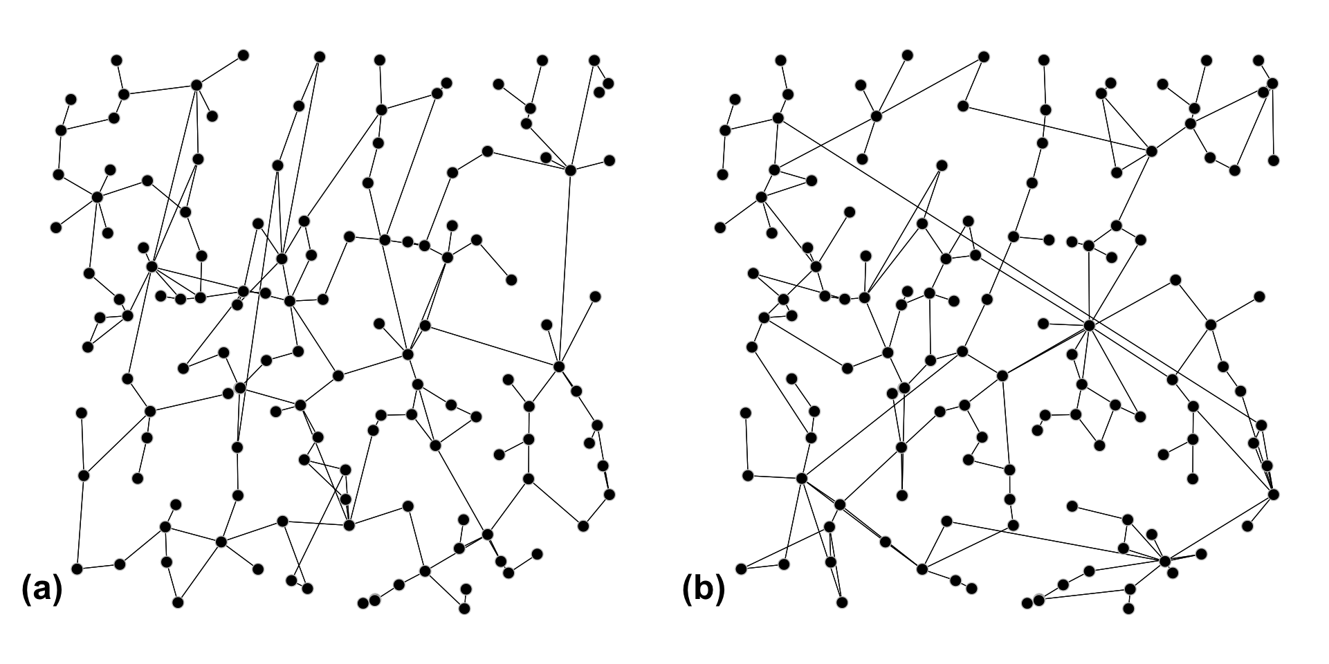Visualisation of two grids generated using the procedure described here. Notice that both present the same bus locations, as their placement is entirely deterministic. The transmission line topology however is different in each case, as it is generated through an stochastic process. Note that the generated grids are non-planar.

The last bus of the list corresponds to a generator (GenBus). One important thing to notice here is that it contains an attribute called gens, which is an array of Generator-type objects. GenBuses represent power plants, which may (or may not, as is the case here) contain several different generating units. These individual generating units are stored within the gens attribute.

We can also inspect the transmission lines:

julia> length(trans_lines(grid))
167

julia> trans_lines(grid)[1]
TransLine(
	connecting: (LoadBus(
	id=3,
	coords=LatLon(lat=33.889332°, lon=-93.097793°),
	load=8.18
	voltage=100,
	population=4090,
	connected_to=Set{Bus}(...)
	connections=Set{TransLine}(...)
), LoadBus(
	id=1,
	coords=LatLon(lat=33.71503°, lon=-93.166445°),
	load=0.17400000000000002
	voltage=200,
	population=87,
	connected_to=Set{Bus}(...)
	connections=Set{TransLine}(...)
)),
	impedance=0.9175166312451004,
	capacity=1400
)

There are 167 transmission lines in our grid. By looking at the first one, we see that they are defined by a tuple of Bus-type objects (here both are LoadBuses), by an impedance value (here taken as Real, since the package has been developed with DC OPF in mind), and a current carrying capacity value.

The adjacency matrix of the system can also be easily accessed:

julia> adjacency(grid)
137×137 SparseMatrixCSC{Bool,Int64} with 334 stored entries:
  [3  ,   1]  =  true
  [6  ,   1]  =  true
  [15 ,   1]  =  true
  [34 ,   1]  =  true
  [35 ,   1]  =  true
  [4  ,   2]  =  true
  ⋮
  [54 , 135]  =  true
  [58 , 135]  =  true
  [67 , 135]  =  true
  [73 , 136]  =  true
  [42 , 137]  =  true
  [46 , 137]  =  true

Notice that we use a sparse matrix representation for better efficiency.

Substations can also be inspected, but we did not create any, so the result should be empty:

julia> substations(grid)
0-element Array{SyntheticGrids.Substation,1}

That can be remedied by changing the boolean value when creating the grid:

julia> grid = Grid(true);

julia> length(substations(grid))
43

julia> substations(grid)[end]
Substation(
	id=43
	coords=LatLon(lat=34.412130070351765°, lon=-93.11856562311557°),
	voltages=Real[115.0],
	load=0,
	generation=199.0,
	population=0,
	connected_to=Set{Substation}(...)
	grouping=SyntheticGrids.Bus[GenBus(
	id=137
	coords=LatLon(lat=34.4425°, lon=-93.0262°),
	generation=56.0
	voltage=Real[115.0],
	tech_type=AbstractString["Conventional Hydroelectric"],
	connected_to=Set{Bus}(...)
	connections=Set{TransLine}(...)
	pfactor=0.9
	summgen=61.8
	wintgen=62.0
	gens=SyntheticGrids.Generator[SyntheticGrids.Generator(LatLon(lat=34.4425°, lon=-93.0262°), Real[115.0], "Conventional Hydroelectric", 28.0, 0.9, 15.0, 30.9, 31.0, "1H", "OP"), SyntheticGrids.Generator(LatLon(lat=34.4425°, lon=-93.0262°), Real[115.0], "Conventional Hydroelectric", 28.0, 0.9, 15.0, 30.9, 31.0, "1H", "OP")]
), GenBus(
	id=135
	coords=LatLon(lat=34.570984°, lon=-93.194425°),
	generation=75.0
	voltage=Real[115.0],
	tech_type=AbstractString["Conventional Hydroelectric"],
	connected_to=Set{Bus}(...)
	connections=Set{TransLine}(...)
	pfactor=0.9
	summgen=75.0
	wintgen=75.0
	gens=SyntheticGrids.Generator[SyntheticGrids.Generator(LatLon(lat=34.570984°, lon=-93.194425°), Real[115.0], "Conventional Hydroelectric", 37.5, 0.9, 20.0, 37.5, 37.5, "10M", "OP"), SyntheticGrids.Generator(LatLon(lat=34.570984°, lon=-93.194425°), Real[115.0], "Conventional Hydroelectric", 37.5, 0.9, 20.0, 37.5, 37.5, "10M", "OP")]
), GenBus(
	id=136
	coords=LatLon(lat=34.211913°, lon=-93.110963°),
	generation=68.0
	voltage=Real[115.0],
	tech_type=AbstractString["Hydroelectric Pumped Storage", "Conventional Hydroelectric"],
	connected_to=Set{Bus}(...)
	connections=Set{TransLine}(...)
	pfactor=0.95
	summgen=68.0
	wintgen=68.0
	gens=SyntheticGrids.Generator[SyntheticGrids.Generator(LatLon(lat=34.211913°, lon=-93.110963°), Real[115.0], "Conventional Hydroelectric", 40.0, 0.95, 15.0, 40.0, 40.0, "1H", "OP"), SyntheticGrids.Generator(LatLon(lat=34.211913°, lon=-93.110963°), Real[115.0], "Hydroelectric Pumped Storage", 28.0, 0.95, 15.0, 28.0, 28.0, "1H", "OP")]
)]
)

By changing the boolean value to true we now create substations (with default values; more into that later) and can inspect them.

A more complete workflow

Let’s now build a grid step by step. First, we start by generating an empty grid:

julia> using SyntheticGrids

julia> grid = Grid()
SyntheticGrids.Grid(2872812514497267479, SyntheticGrids.Bus[], SyntheticGrids.TransLine[], SyntheticGrids.Substation[], Array{Bool}(0,0), Array{Int64}(0,0))

Notice that one of the attributes has been automatically initialised. That corresponds to the seed which will be used for all stochastic steps. Control over the seed value gives us control over reproducibility. Conversely, that value could have been specified via grid = Grid(seed).

Now let’s place the load buses. We could do this by specifying latitude and longitude limits (e.g.: place_loads_from_zips!(grid; latlim = (30, 35), longlim = (-99, -90))), but let’s look at a more general way of doing this. We can define any function that receives a tuple containing a latitude–longitude pair and returns true if within the desired region and false otherwise:

julia> my_region(x::Tuple{Float64, Float64}, r::Float64) = ((x[1] - 33)^2 + (x[2] + 95)^2 < r^2)
my_region (generic function with 1 method)

julia> f(x) = my_region(x, 5.)
f (generic function with 1 method)

julia> place_loads_from_zips!(grid, f)

julia> length(buses(grid))
3287

Here, my_region defines a circle (in latitude-longitude space) of radius r around the point (33, -95). Any zip code within that region is added to the grid (to a total of 3287) as a load bus. The same can be done for the generators:

julia> place_gens_from_data!(grid, f)

julia> length(buses(grid))
3729

This command adds all generators within the same region, bringing the total amount of buses to 3729.

We can also manually add extra load or generation buses if we wish:

julia> a_bus = LoadBus((22., -95.), 12., 200, 12345)
LoadBus(
	id=-1,
	coords=LatLon(lat=22.0°, lon=-95.0°),
	load=12.0
	voltage=200,
	population=12345,
	connected_to=Set{Bus}()
	connections=Set{Transline}()
)

julia> SyntheticGrids.add_bus!(grid, a_bus)

julia> length(buses(grid))
3730

The same works for GenBuses.

Once all buses are in place, it is time to connect them with transmission lines. This can be done via a single function (this step can take some time for larger grids):

julia> connect!(grid)

julia> length(trans_lines(grid))
0

This function goes through the stochastic process of creating the system’s adjacency matrix, but it does not create the actual TransLine objects (hence the zero length). That is done via the create_lines! function. Also note that connect! has several parameters for which we adopted default values. For a description of those, see ? connect.

Before we create the lines, it is interesting to revisit adding new buses. Now that we have created the adjacency matrix for the network, we have two options when adding a new bus: either we redo the connect! step in order to incorporate the new bus in the grid, or we simply extend the adjacency matrix to include the new bus (which won’t have any connections). This is controlled by the reconnect keyword argument that can be passed to add_bus!. In the former case, one uses reconnect = false (the default option); connections can always be manually added by editing the adjacency matrix (and the connected_to fields of the involved buses).

Once the adjacency matrix is ready, TransLine objects are created by invoking the create_lines! function:

julia> SyntheticGrids.create_lines!(grid)

julia> length(trans_lines(grid))
4551

We have generated the connection topology with transmission line objects. Finally, we may want to coarse-grain the grid. This is done via the cluster! function, which receives as arguments the number of each type of cluster: load, both load and generation or pure generation. This step may also take a little while for large grids.

julia> length(substations(grid))
0

julia> cluster!(grid, 1500, 20, 200)

julia> length(substations(grid))
1700

At this point, the whole grid has been generated. If you wish to save it, the functions save and load_grid are available. Please note that the floating-point representation of numbers may lead to infinitesimal changes to the values when saving and reloading a grid. Besides precision issues, they should be equivalent.

julia> save(grid, "./test_grid.json")

julia> grid2 = load_grid("./test_grid.json")

Some simple statistics can be computed over the grid, such as the average node degree and the clustering coefficient:

julia> mean_node_deg(adjacency(grid))
2.4402144772117964

julia> cluster_coeff(adjacency(grid))
0.08598360707539486

The generated grid can easily be exported to pandapower in order to carry out powerflow studies. The option to export to PowerModels.jl should be added soon.

julia> pgrid = to_pandapower(grid)
PyObject This pandapower network includes the following parameter tables:
   - load (3288 elements)
   - trafo (913 elements)
   - ext_grid (1 elements)
   - bus_geodata (3730 elements)
   - bus (3730 elements)
   - line (3638 elements)
   - gen (1397 elements)

Conclusion

Hopefully, this post helped as a first introduction to the SyntheticGrids.jl package. There are more functions which have not been mentioned here; the interested reader should refer to the full documentation for a complete list of methods. This is an ongoing project, and, as such, several changes and additions might still happen. The most up-to-date version can always be found at Github.