In software development, the term “deprecated” refers to functionality that is still usable, but is obsolete and about to be replaced or removed in a future version of the software.
This blog post will explain why deprecating functionality is a good idea, and will discuss available mechanisms for deprecating functionality in the Julia language.
Why deprecate?
An important aspect of software development is minimising the pain of users.
Making few breaking changes to the API goes a long way towards pain minimisation, but sometimes breaking changes are necessary.
Although following the semantic versioning rules SemVer will alert the users of a breaking change by incrementing the major version, the users still need to figure out the changes that need to be made in their code in order to support the new version of your software.
They can do so by going through the release notes, if such notes are provided, or by running the tests and hoping they have good coverage.
Deprecations are a way to make this easier, by releasing a non-breaking version of the software before releasing the breaking version.
In the non-breaking version, the functionality to be removed emits warnings when used, and the warnings describe how to update the code to work in the breaking version.
How to deprecate in Julia
The following workflow is recommended:
Move the deprecated functionality to a file named src/deprecated.jl, and deprecate it (see section below for details on how to do this).
Move the tests for deprecated functionality to test/deprecated.jl.
Release a non-breaking version of your package.
Using this non-breaking release will emit deprecation warnings when deprecated functionality is used, guiding users to make the right changes in their code.
Once you are ready to make a breaking release:
Delete the src/deprecated.jl file
Delete the test/deprecated.jl file
Release a breaking version of your package
Note that for more complex breaking changes it may be more practical to not spend too much time on complicated deprecation setups, and instead just produce a written upgrading guide.
The rest of the post describes the private methods available in Julia Base to help with the deprecations.
Base.@deprecate
If you’ve simply renamed a function or changed the signature without modifying the underlying behaviour then you should use the Base.@deprecate macro:
The example above will inform the users that a keyword argument was renamed, and advises how to change the call signature.
NOTE:Base.@deprecate will export the symbol being deprecated by default, but you can disable that behaviour by adding false to the end of you statement:
If you’re deprecating a symbol from your package (e.g. renaming a type) then you should use the @deprecate_binding macro:
Base.@deprecate_bindingMyOldTypeMyNewType
If you are removing a function without methods (like function bar end) that is typically overloaded, then you can use:
Base.@deprecate_bindingbarnothing
Base.@deprecate_moved
If you’re deprecating a symbol from your package because it has simply been moved to another package, then you can use the @deprecate_moved macro to give an informative error:
Base.@deprecate_movedMyTrustyType"OtherPackage"
Base.depwarn
If you’re introducing other breaking changes that do not fall in any of the above categories, you can use Base.depwarn and write a custom deprecation warning.
An example would be deprecating a type parameter:
function MyType{G}(args...)whereGBase.depwarn("The `G` type parameter will be deprecated in a future release. "*"Please use `MyType(args...)` instead of `MyType{$G}(args...)`.",:MyType,)returnMyType(args...)end
Unlike other methods of deprecation, Base.depwarn has a force keyword argument that will cause it to be shown even if Julia is run with (the default) --depwarn=false.
Tempting as it is, we advise against using it in most circumstances, because there is a good reason deprecations are not shown.
Printing a warning in the module __init__() is a similar option that should almost never be used.
Warnings in module __init__()
If you’re making broad changes at the module level (e.g., removing exports, changes to defaults/constants) you may simply want to throw a warning when the package loads.
However, this should be a last resort, as it makes a lot of noise, often in unexpected places (e.g downstream dependents).
# Example from Impute.jlfunction __init__()sym=join(["chain","chain!","drop","drop!","interp","interp!"],", "," and ")@warn("""
The following symbols will not be exported in future releases: $sym.
Please qualify your calls with `Impute.<method>(...)` or explicitly import the symbol.
""")@warn("""
The default limit for all impute functions will be 1.0 going forward.
If you depend on a specific threshold please pass in an appropriate `AbstractContext`.
""")@warn("""
All matrix imputation methods will be switching to the JuliaStats column-major convention
(e.g., each column corresponds to an observation, and each row corresponds to a variable).
""")end
When are deprecations shown in Julia?
Since Julia 1.5 (PR #35362) deprecations have been muted by default.
They are only shown if Julia is started with the --depwarn=yes flag set.
The reason for this has two main parts.
The practical reason is the deprecation logging itself is quite slow and so by calling a deprecated method in an inner loop some packages were becoming unusably slow, thus making the deprecation effectively breaking.
The logical reason is the user of a package often can’t fix them (unless called directly), they often need to be fixed in some downstream dependency of the package they are using.
Thanks to Julia packages following SemVer, calling a deprecated method is completely safe, until you relax the bounds.
When relaxing the compat bound it is good practice to check the release notes, relax the compat bounds and then run integration tests.
If everything passes then you are done, if not retighten the compat bounds and run with --depwarn=error (or pay careful attention to logs) and track them down.
Deprecations are by default shown during tests.
This is because tests are run mostly by the developers of the package.
However, they still may be unfixable by the developer of the package if they are downstream, but at least the developer is probably in a better position to open PRs or issues in their dependencies.
Internally at Invenia, we take a different approach.
Because deprecations are so spammy we also disable them in our main CI runs.
But we have an additional CI job that is set to --depwarn=error, with allowed-to-fail set on the job.
This keeps the logs in our main CI clean, while also quickly alerting us if any deprecated methods are hit.
Conclusions
Deprecating package functionality is a bit of work, but it minimises the amount of pain for package users when breaking changes are released.
The recommended workflow in Julia includes moving all the deprecated functionality and its tests into dedicated deprecated.jl files, which makes it easier to remove once the breaking version is released.
Julia offers several convenience macros in Base which make common operations like changing a function signature, moving functionality, or renaming types a one-line operation.
For more complicated changes a custom message can be written.
Deprecation warnings are suppressed in Julia by default for performance reasons, but they can be shown by setting the --depwarn=true flag when starting a new Julia session.
In a previous blog post, we reviewed how neural networks (NNs) can be used to predict solutions of optimal power flow (OPF) problems.
We showed that widely used approaches fall into two major classes: end-to-end and hybrid techniques.
In the case of end-to-end (or direct) methods, a NN is applied as a regressor and either the full set or a subset of the optimization variables is predicted based on the grid parameters (typically active and reactive power loads).
Hybrid (or indirect) approaches include two steps: in the first step, some of the inputs of OPF are inferred by a NN, and in the second step an OPF optimization is performed with the predicted inputs.
This can reduce the computational time by either enhancing convergence to the solution or formulating an equivalent but smaller problem.
Under certain conditions, hybrid techniques provide feasible (and sometimes even optimal) values of the optimization variables of the OPF.
Therefore, hybrid approaches constitute an important research direction in the field.
However, feasibility and optimality have their price: because of the requirement of solving an actual OPF, hybrid methods can be computationally expensive, especially when compared to end-to-end techniques.
In this blog post, we discuss an approach to minimize the total computational time of hybrid methods by applying a meta-objective function that directly measures this computational cost.
Hybrid NN-based methods for predicting OPF solutions
In this post we will focus solely on hybrid NN-based methods.
For more detailed theoretical background we suggest reading our earlier blog post.
OPF problems are mathematical optimizations with the following concise and generic form:
where \(x\) is the vector of grid parameters and \(y\) is the vector of optimization variables, \(f(x, y)\) is the objective (or cost) function to minimize, subject to equality constraints \(c_{i}^{\mathrm{E}}(x, y) \in \mathcal{C}^{\mathrm{E}}\) and inequality constraints \(c_{j}^{\mathrm{I}}(x, y) \in \mathcal{C}^{\mathrm{I}}\).
For convenience we write \(\mathcal{C}^{\mathrm{E}}\) and \(\mathcal{C}^{\mathrm{I}}\) for the sets of equality and inequality constraints, with corresponding cardinalities \(n = \lvert \mathcal{C}^{\mathrm{E}} \rvert\) and \(m = \lvert \mathcal{C}^{\mathrm{I}} \rvert\), respectively.
This optimization problem can be non-linear, non-convex, and even mixed-integer.
The most widely used approach to solving it is the interior-point method.123
The interior-point method is based on an iteration, which starts from an initial value of the optimization variables (\(y^{0}\)).
At each iteration step, the optimization variables are updated based on the Newton-Raphson method until some convergence criteria have been satisfied.
OPF can be also considered as an operator4 that maps the grid parameters (\(x\)) to the optimal value of the optimization variables (\(y^{*}\)).
In a more general sense (Figure 1), the objective and constraint functions, as well as the initial value of the optimization variables, are also arguments of this operator and we can write:
where \(\Omega\) is an abstract set within the values of the operator arguments are allowed to change and \(n_{y}\) is the dimension of the optimization variables.
Hybrid NN-based techniques apply neural networks to predict some arguments of the operator in order to reduce the computational time of running OPF compared to default methods.
Figure 1. OPF as an operator.
Regression-based hybrid methods
Starting the optimization from a specified value of the optimization variables (rather than the default used by a given solver) in the framework of interior-point methods is called warm-start optimization.
Directly predicting the optimal values of the optimization variables (end-to-end or direct methods) can result in a sub-optimal or even infeasible point.
However, as it is presumably close enough to the solution, it seems to be a reasonable approach to use this predicted value as the starting point of a warm-start optimization.
Regression-based indirect techniques follow exactly this route56: for a given grid parameter vector \(x_{t}\), a NN is applied to obtain the predicted set-point, \(\hat{y}_{t}^{0} = \mathrm{NN}_{\theta}^{\mathrm{r}}(x_{t})\), where the subscript \(\theta\) denotes all parameters (weights, biases, etc.) of the NN, and the superscript \(\mathrm{r}\) indicates that the NN is used as a regressor.
Based on the predicted set-point, a warm-start optimization can be performed:
Warm-start methods provide an exact (locally) optimal point, as the solution is eventually obtained from an optimization problem identical to the original one.
Training the NN is performed by minimizing the sum (or mean) of some differentiable loss function of the training samples with respect to the NN parameters:
where \(N_{\mathrm{train}}\) denotes the number of training samples and \(L^{\mathrm{r}} \left(y_{t}^{*}, \hat{y}_{t}^{(0)} \right)\) is the (regression) loss function between the true and predicted values of the optimal point.
Typical loss functions are the (mean) squared error, \(SE \left(y_{t}^{*}, \hat{y}_{t}^{(0)} \right) = \left\| y_{t}^{*} - \hat{y}_{t}^{(0)} \right\|^{2}\), and (mean) absolute error, \(AE \left(y_{t}^{*}, \hat{y}_{t}^{(0)} \right) = \left\| y_{t}^{*} - \hat{y}_{t}^{(0)} \right\|\) functions.
Figure 2. Flowchart of the warm-start method (yellow panel) in combination with an NN regressor (purple panel, default arguments of OPF operator are omitted for clarity) trained by minimizing a conventional loss function.
Classification-based hybrid methods
An alternative hybrid approach using a NN classifier (\(\mathrm{NN}_{\theta}^{\mathrm{c}}\)) leverages the observation that only a fraction of all constraints is binding at the optimum78, so a reduced OPF problem can be formulated by keeping only the binding constraints.
Since this reduced problem still has the same objective function as the original one, the solution should be equivalent to that of the original full
problem: \(\Phi \left( x_{t}, y^{0}, f, \mathcal{C}^{\mathrm{E}}, \mathcal{A}_{t} \right) = \Phi \left( x_{t}, y^{0}, f, \mathcal{C}^{\mathrm{E}}, \mathcal{C}^{\mathrm{I}} \right) = y_{t}^{*}\), where \(\mathcal{A}_{t} \subseteq \mathcal{C}^{\mathrm{I}}\) is the active or binding subset of the inequality constraints (also note that \(\mathcal{C}^{\mathrm{E}} \cup \mathcal{A}_{t}\) contains all active constraints defining the specific congestion regime).
This suggests a classification formulation in which the grid parameters are used to predict the active set:
Technically, the NN can be used in two ways to predict the active set.
One approach is to identify all distinct active sets in the training data and train a multiclass classifier that maps the input to the corresponding active set.8
Since the number of active sets increases exponentially with system size, for larger grids it might be better to predict the binding status of each non-trivial constraint by using a binary multi-label classifier.9
However, since the classifiers are not perfect, there may be violated constraints not included in the reduced model.
One of the most widely used approaches to ensure convergence to an optimal point of the full problem is the iterative feasibility test.109
The procedure has been widely used by power grid operators and it includes the following steps in combination with a classifier:
An initial active set of inequality constraints (\(\hat{\mathcal{A}}_{t}^{(1)}\)) is proposed by the classifier and a solution of the reduced problem is obtained.
In each feasibility iteration, \(k = §1, \ldots, K\), the optimal point of the actual reduced problem (\({\hat{y}_{t}^{*}}^{(k)}\)) is validated against the constraints \(\mathcal{C}^{\mathrm{I}}\) of the original full formulation.
At each step \(k\), the violated constraints \(\mathcal{N}_{t}^{(k)} \subseteq \mathcal{C}^{\mathrm{I}} \setminus \hat{\mathcal{A}}_{t}^{(k)}\) are added to the set of considered inequality constraints to form the active set of the next iteration: \(\hat{\mathcal{A}}_{t}^{(k+1)} = \hat{\mathcal{A}}_{t}^{(k)} \cup \mathcal{N}_{t}^{(k)}\).
The procedure repeats until no violations are found (i.e. \(\mathcal{N}_{t}^{(k)} = \emptyset\)), and the optimal point satisfies all original constraints \(\mathcal{C}^{\mathrm{I}}\). At this point, we have found the optimal point to the full problem (\({\hat{y}_{t}^{*}}^{(k)} = y_{t}^{*}\)).
As the reduced OPF is much cheaper to solve than the full problem, this procedure (if converged in few iterations) can be in theory very efficient, resulting in an optimal solution to the full OPF problem.
Obtaining optimal NN parameters is again based on minimizing a loss function of the training data:
where \(L^{\mathrm{c}} \left( \mathcal{A}_{t}, \hat{\mathcal{A}}_{t}^{(1)} \right)\) is the classifier loss as a function of the true and predicted active inequality constraints.
For instance, for predicting the binding status of each potential constraint, the typical loss function used is the binary cross-entropy: \(BCE \left( \mathcal{A}_{t}, \hat{\mathcal{A}}_{t}^{(1)} \right) = -\frac{1}{m} \sum \limits_{j=1}^{m} c^{(t)}_{j} \log \hat{c}^{(t)}_{j} + \left( 1 - c^{(t)}_{j} \right) \log \left( 1 - \hat{c}^{(t)}_{j} \right)\), where \(c_{j}^{(t)}\) and \(\hat{c}_{j}^{(t)}\) are the true value and predicted probability of the binding status of the \(j\)th inequality constraint.
Figure 3. Flowchart of the iterative feasibility test method (yellow panel) in combination with a NN classifier (purple panel; default arguments of OPF operator are omitted for clarity) trained by minimizing a conventional loss function.
Meta-loss
In the previous sections, we discussed hybrid methods that apply a NN either as a regressor or a classifier to predict starting values of the optimization variables and initial set of binding constraints, respectively, for the subsequent OPF calculations.
During the optimization of the NN parameters some regression- or classification-based loss function of the training data is minimized.
However, below we will show that these conventional loss functions do not necessarily minimize the most time consuming part of the hybrid techniques, i.e. the computationally expensive OPF step(s).
Therefore, we suggest a meta-objective function that directly addresses this computational cost.
Meta-optimization for regression-based hybrid approaches
Conventional supervised regression techniques typically use loss functions based on a distance between the training ground-truth and predicted output
value, such as mean squared error or mean absolute error.
In general, each dimension of the target variable is treated equally in these loss functions.
However, the shape of the Lagrangian landscape of the OPF problem as a function of the optimization variables is far from isotropic11, implying that optimization under such an objective does not necessarily minimize the warm-started OPF solution time.
Also, trying to derive initial values for optimization variables using empirical risk minimization techniques does not guarantee feasibility, regardless of the accuracy of the prediction to the ground truth.
Interior-point methods start by first moving the system into a feasible region, thereby potentially altering the initial position significantly. Consequently, warm-starting from an infeasible point can be inefficient.
Instead, one can use a meta-loss function that directly measures the computational cost of solving the (warm-started) OPF problem.69
One measure of the computational cost can be defined by the number of iterations \((N(\hat{y}^{0}_{t}))\) required to reach the optimal solution.
Since the warm-started OPF has exactly the same formulation as the original OPF problem, the comparative number of iterations represents the improvement in computational cost.
Alternatively, the total CPU time of the warm-started OPF \((T(\hat{y}^{0}_{t}))\) can also be measured, although, unlike the number of iterations, it is not a noise-free measure.
Figure 4 presents a flowchart of the procedure for using a NN with parameters determined by minimizing the computational time-based meta-loss function (meta-optimization) on the training set.
As this meta-loss is a non-differentiable function with respect to the NN weights, back-propagation cannot be used.
As an alternative, one can employ gradient-free optimization techniques.
Figure 4. Flowchart of the warm-start method (yellow panel) in combination with an NN regressor (purple panel; default arguments of the OPF operator are omitted for clarity) trained by minimizing a meta-loss function that is a sum of the computational time of warm-started OPFs of the training data.
Meta-optimization for classification-based hybrid approaches
In the case of the classification-based hybrid methods, the goal is to find NN weights that minimize the total computational time of the iterative feasibility test.
However, minimizing a cross-entropy loss function to obtain such weights is not straightforward.
First, the number of cycles in the iterative procedure is much more sensitive to false negative than to false positive predictions of the binding
status.
Second, different constraints can be more or less important depending on the actual congestion regime and binding status (Figure 5).
These suggest the use of a more sophisticated objective function, for instance a weighted cross-entropy with appropriate weights for the corresponding terms.
The weights as hyperparameters can then be optimized to achieve an objective that can adapt to the above requirements.
However, an alternative objective can be defined as the total computational time of the iterative feasibility test procedure.9
Figure 5. Profile of the meta-loss (total computational time) and number of iterations within the iterative feasibility test as functions of the number of constraints for two grids, and a comparison of DC vs. AC formulations. Perfect classifiers with the active set (AS) are indicated by vertical dashed lines, with the false positive (FP) region to the right, and the false negative (FN) region to the left.9
The meta-loss objective, therefore, includes the solution time of a sequence of reduced OPF problems.
Similarly to the meta-loss defined for the regression approach, it measures the computational cost of obtaining a solution of the full problem and, unlike weighted cross-entropy, it does not require additional hyperparameters to be optimized.
Figure 6. Flowchart of the iterative feasibility test method (yellow panel) in combination with an NN classifier (purple panel; default arguments of the OPF operator are omitted for clarity) trained by minimizing a meta-loss function that is a sum of the computational time of the iterative feasibility tests of the training data.
Optimizing the meta-loss function: the particle swarm optimization method
Neither the number of iterations nor the computational time of the subsequent OPF is a differentiable quantity with respect to the applied NNs.
Therefore, to obtain optimal NN weights by minimizing the meta-loss, a gradient-free method (i.e. using only the value of the loss function) is required.
The particle swarm optimization was found to be a particularly promising9 gradient-free approach for this.
Particle swarm optimization (PSO) is a gradient-free meta-heuristic algorithm inspired by the concept of swarm intelligence that can be found in nature within certain animal groups.
The method applies a set of particles (\(N_{\mathrm{p}}\)) and the particle dynamics at each optimization step is influenced by both the individual (best position found by the particle) and collective (best position found among all particles) knowledge.
More specifically, for a \(D\) dimensional problem, each particle \(p\) is associated with a velocity \(v^{(p)} \in \mathbb{R}^{D}\) and position \(x^{(p)} \in \mathbb{R}^{D}\) vectors that are randomly initialized at the beginning of the optimization within the corresponding ranges of interest.
During the course of the optimization, the velocities and positions are updated and in the \(n\)th iteration, the new vectors are obtained as12:
where \(\omega_{n}\) is the inertia weight, \(c_{1}\) and \(c_{2}\) are the acceleration coefficients, \(r_{n}\) and \(q_{n}\) are random vectors whose each component is drawn from a uniform distribution within the \([0, 1]\) interval, \(l_{n}^{(p)}\) is the best local position found by particle \(p\) and \(g_{n}\) is the best global position found by all particles together so far, and \(\odot\) denotes the Hadamard (pointwise) product.
As it seems from eq. \ref{eq:pso}, PSO is a fairly simple approach: the particles’ velocity is governed by three terms: inertia, local and global knowledge.
The method was originally proposed for global optimization and it can be easily parallelized across the particles.
Numerical experiments
We demonstrate the increased performance of the meta-loss objective compared to conventional loss functions for the classification-based hybrid approach.
Three synthetic grids using both DC and AC formulations were investigated using 10k and 1k samples, respectively.
The samples were split randomly into training, validation, and test sets containing 70%, 20%, and 10% of the samples, respectively.
A fully connected NN was trained using a conventional and a weighted cross-entropy objective function in combination with a standard gradient-based optimizer (ADAM).
As discussed earlier, the meta-loss is much more sensitive to false negative predictions (Figure 5).
To reflect this in the weighted cross-entropy expression, we applied weights of 0.25 and 0.75 for the false positive and false negative penalty terms.
Then, starting from these optimized NNs, we performed further optimizations, using the meta-loss objective in combination with a PSO optimizer.
Table 1 includes the average computational gains (compared to the full problem) of the different approaches using 10 independent experiments for each.
For all cases, the weighted cross-entropy objective outperforms the conventional cross-entropy, indicating the importance of the false negative penalty term.
However, optimizing the NNs further by the meta-loss objective significantly improves the computational gain for both cases.
For AC-OPF, it brings the gain into the positive regime.
For details on how to use a meta-loss function, as well as for further numerical results, we refer to our paper.9
Table 1. Average gain with two sided \(95\)% confidence intervals of classification-based hybrid models in combination with meta-optimization using conventional and weighted binary cross-entropy for pre-training the NN.
Case
Gain (%)
Conventional
Weighted
Cross-entropy
Meta-loss
Cross-entropy
Meta-loss
DC-OPF
118-ieee
$$\begin{equation*}38.2 \pm 0.8\end{equation*}$$
$$\begin{equation*}42.1 \pm 2.7\end{equation*}$$
$$\begin{equation*}43.0 \pm 0.5\end{equation*}$$
$$\begin{equation*}44.8 \pm 1.2\end{equation*}$$
162-ieee-dtc
$$\begin{equation*}8.9 \pm 0.9\end{equation*}$$
$$\begin{equation*}31.2 \pm 1.3\end{equation*}$$
$$\begin{equation*}21.2 \pm 0.7\end{equation*}$$
$$\begin{equation*}36.9 \pm 1.0\end{equation*}$$
300-ieee
$$\begin{equation*}-47.1 \pm 0.5\end{equation*}$$
$$\begin{equation*}11.8 \pm 5.2\end{equation*}$$
$$\begin{equation*}-10.2 \pm 0.8\end{equation*}$$
$$\begin{equation*}23.2 \pm 1.8\end{equation*}$$
AC-OPF
118-ieee
$$\begin{equation*}-31.7 \pm 1.2\end{equation*}$$
$$\begin{equation*}20.5 \pm 4.2\end{equation*}$$
$$\begin{equation*}-3.8 \pm 2.3\end{equation*}$$
$$\begin{equation*}29.3 \pm 2.0\end{equation*}$$
162-ieee-dtc
$$\begin{equation*}-60.5 \pm 2.7\end{equation*}$$
$$\begin{equation*}8.6 \pm 7.6\end{equation*}$$
$$\begin{equation*}-28.4 \pm 3.0\end{equation*}$$
$$\begin{equation*}23.4 \pm 2.2\end{equation*}$$
300-ieee
$$\begin{equation*}-56.0 \pm 5.8\end{equation*}$$
$$\begin{equation*}5.0 \pm 6.4\end{equation*}$$
$$\begin{equation*}-30.9 \pm 2.2\end{equation*}$$
$$\begin{equation*}15.8 \pm 2.3\end{equation*}$$
Conclusion
NN-based hybrid approaches can guarantee optimal solutions and are therefore a particularly interesting research direction among machine learning assisted OPF models.
In this blog post, we argued that the computational cost of the subsequent (warm-start or set of reduced) OPF can be straightforwardly reduced by applying a meta-loss objective.
Unlike conventional loss functions that measure some error between the ground truth and the predicted quantities, the meta-loss objective directly addresses the computational time.
Since the meta-loss is not a differentiable function of the NN weights, a gradient-free optimization technique, like the particle swarm optimization approach, can be used.
Although significant improvements of the computational cost of OPF can be achieved by applying a meta-loss objective compared to conventional loss functions, in practice these gains are still far from desirable (i.e. the total computational cost should be a fraction of that of the original OPF problem).9
In a subsequent blog post, we will discuss how neural networks can be utilized in a more efficient way to obtain optimal OPF solutions.
S. Boyd and L. Vandenberghe, “Convex Optimization”, New York: Cambridge University Press, (2004). ↩
M. Jamei, L. Mones, A. Robson, L. White, J. Requeima and C. Ududec, “Meta-Optimization of Optimal Power Flow”, Proceedings of the 36th International Conference on Machine Learning Workshop, (2019) ↩↩2
Z. Zhan, J. Zhang, Y. Li and H. S. Chung, “Adaptive particle swarm optimization”, IEEE Transactions on Systems, Man, and Cybernetics, Part B (Cybernetics), 39, 1362, (2009). ↩
In a previous blog post, we discussed the fundamental concepts of optimal power flow (OPF), a core problem in operating electricity grids.
In their principal form, AC-OPFs are non-linear and non-convex optimization problems that are in general expensive to solve.
In practice, due to the large size of electricity grids and number of constraints, solving even the linearized approximation (DC-OPF) is a challenging optimization requiring significant computational effort.
Adding to the difficulty, the growing integration of renewable generation has increased uncertainty in grid conditions and increasingly requires grid operators to solve OPF problems in near real-time.
This has led to new research efforts in using machine learning (ML) approaches to shift the computational effort away from real-time (optimization) to offline training, potentially providing an almost instant prediction of the outputs of OPF problems.
This blog post focuses on a specific set of machine learning approaches that applies neural networks (NNs) to predict (directly or indirectly) solutions to OPF.
In order to provide a concise and common framework for these approaches, we consider first the general mathematical form of OPF and the standard technique to solve it: the interior-point method.
Then, we will see that this optimization problem can be viewed as an operator that maps a set of quantities to the optimal value of the optimization variables of the OPF.
For the simplest case, when all arguments of the OPF operator are fixed except the grid parameters, we introduce the term, OPF function.
We will show that all the NN-based approaches discussed here can be considered as estimators of either the OPF function or the OPF operator.1
General form of OPF
OPF problems can be expressed in the following concise form of mathematical programming:
where \(x\) is the vector of grid parameters and \(y\) is the vector of optimization variables, \(f(x, y)\) is the objective (or cost) function to minimize, subject to equality constraints \(c_{i}^{\mathrm{E}}(x, y) \in \mathcal{C}^{\mathrm{E}}\) and inequality constraints \(c_{j}^{\mathrm{I}}(x, y) \in \mathcal{C}^{\mathrm{I}}\).
For convenience we write \(\mathcal{C}^{\mathrm{E}}\) and \(\mathcal{C}^{\mathrm{I}}\) for the sets of equality and inequality constraints, respectively, with corresponding cardinalities \(n = \lvert \mathcal{C}^{\mathrm{E}} \rvert\) and \(m = \lvert \mathcal{C}^{\mathrm{I}} \rvert\).
The objective function is optimized solely with respect to the optimization variables (\(y\)), while variables (\(x\)) parameterize the objective and constraint functions.
For example, for a simple economic dispatch (ED) problem \(x\) includes voltage magnitudes and active powers of generators, \(y\) is a vector of active and reactive power components of loads, the objective function is the cost of the total real power generation, equality constraints include the power balance and power flow equations, while inequality constraints impose lower and upper bounds on other critical quantities.
The most widely used approach to solving the above optimization problem (that can be non-linear, non-convex and even mixed-integer) is the interior-point method.234
The interior-point (or barrier) method is a highly efficient iterative algorithm.
However, it requires the computation of the Hessian (i.e. second derivatives) of the Lagrangian of the system with respect to the optimization variables at each iteration step.
Due to the non-convex nature of the power flow equations appearing in the equality constraints, the method can be prohibitively slow for large-scale systems.
The formulation of eq. \(\eqref{opt}\) gives us the possibility of looking at OPF as an operator that maps the grid parameters (\(x\)) to the optimal value of the optimization variables (\(y^{*}\)).
In a more general sense, the objective and constraint functions are also arguments of this operator.
Also, in this discussion we assume that, if feasible, the exact solution of the OPF problem is always provided by the interior-point method.
Therefore, the operator is parameterized implicitly by the starting value of the optimization variables (\(y^{0}\)).
The actual value of \(y^{0}\) can significantly affect the convergence rate of the interior-point method and the total computational time, and for non-convex formulations (where multiple local minima might exist) even the optimal point can differ.
The general form of the OPF operator can be written as:
where \(\Omega\) is an abstract set within the values of the operator arguments are allowed to change and \(n_{y}\) is the dimension of the optimization variables.
We note that a special case of the general form is the DC-OPF operator, whose mathematical properties have been thoroughly investigated in a recent work.5
In many recurring problems, most of the arguments of the OPF operator are fixed and only (some of) the grid parameters vary.
For these cases, we introduce a simpler notation, the OPF function:
where \(n_{x}\) and \(n_{y}\) are the dimensions of grid parameter and optimization variables, respectively.
We also denote the set of all feasible points of OPF as \(\mathcal{F}_{\Phi}\).
The optimal value \(y^{*}\) is a member of the set \(\mathcal{F}_{\Phi}\) and in the case when the problem is infeasible, \(\mathcal{F}_{\Phi} = \emptyset\).
The daily task of electricity grid operators is to provide solutions for OPF, given constantly changing grid parameters \(x_{t}\).
The standard OPF approach would be to compute \(F_{\Phi}(x_{t}) = y_{t}^{*}\) using some default values of the other arguments of \(\Phi\).
However, in practice this is used rather rarely as usually additional information about the grid is also available that can be used to obtain the solution more efficiently.
For instance, it is reasonable to assume that for similar grid parameter vectors the corresponding optimal points are also close to each other.
If one of these problems is solved then its optimal point can be used as the starting value for the optimization variables of the other problem, which can then converge significantly faster compared to some default initial values.
This strategy is called warm-start and might be useful for consecutive problems, i.e. \(\Phi \left( x_{t}, y_{t-1}^{*}, f, \mathcal{C}^{\mathrm{E}}, \mathcal{C}^{\mathrm{I}} \right) = y_{t}^{*}\).
Another way to reduce the computational time of solving OPF is to reduce the problem size.
The OPF solution is determined by the objective function and all binding constraints.
However, at the optimal point, not all of the constraints are actually binding and there is a large number of non-binding inequality constraints that can be therefore removed from the mathematical problem without changing the optimal point, i.e. \(\Phi \left( x_{t}, y^{0}, f, \mathcal{C}^{\mathrm{E}}, \mathcal{A}_{t} \right) = y_{t}^{*}\), where \(\mathcal{A}_{t}\) is the set of all binding inequality constraints of the actual problem (equality constraints are always binding).
This formulation is called reduced OPF and it is especially useful for DC-OPF problems.
The three main approaches discussed are depicted in Figure 1.
Figure 1. Main approaches to solving OPF. Varying arguments are highlighted, while other arguments are potentially fixed.
NN-based approaches for predicting OPF solutions
The ML methods we will discuss apply either an estimator function (\(\hat{F}_{\Phi}(x_{t}) = \hat{y}_{t}^{*}\)) or an estimator operator (\(\hat{\Phi}(x_{t}) = \hat{y}_{t}^{*}\)) to provide a prediction of the optimal point of OPF based on the grid parameters.
We can categorize these methods in different ways.
For instance, based on the estimator type they use, we can distinguish between end-to-end (aka direct) and hybrid (aka indirect) approaches.
End-to-end methods use a NN as an estimator function and map the grid parameters directly to the optimal point of OPF.
Hybrid or indirect methods apply an estimator operator that includes two steps: in the first step, a NN maps the grid parameters to some quantities, which are then used in the second step as inputs to some optimization problem resulting in the predicted (or even exact) optimal point of the original OPF problem.
We can also group techniques based on the NN predictor type: the NN can be used either as regressor or classifier.
Regression
The OPF function establishes a non-linear relationship between the grid parameters and optimization variables.
In regression techniques, this complex relationship is approximated by NNs, treating the grid parameters as the input and the optimal values of the optimization variables as the output of the NN model.
End-to-end methods
End-to-end methods6 apply NNs as regressors, mapping the grid parameters (as inputs) directly to the optimal point of OPF (as outputs):
where the subscript \(\theta\) denotes all parameters (weights, biases, etc.) of the NN and the superscript \(\mathrm{r}\) indicates that the NN is used as a regressor.
We note that once the prediction \(\hat{y}_{t}^{*}\) is computed, other dependent quantities (e.g. power flows) can be easily obtained by solving the power flow problem67 — given the prediction is a feasible point.
As OPF is a constrained optimization problem, the optimal point is not necessarily a smooth function of the grid parameters: changes of the binding status of constraints can lead to abrupt changes of the optimal solution.
Also, the number of congestion regimes — i.e. the number of distinct sets of active (binding) constraints — increases exponentially with grid size.
Therefore, in order to obtain sufficiently high coverage and accuracy of the model, a substantial amount of training data is required.
Warm-start methods
For real power grids, the available training data is rather limited compared to the system size.
As a consequence, it is challenging to provide predictions by end-to-end methods that are optimal.
Of even greater concern, there is no guarantee that the predicted optimal point is a feasible point (i.e. satisfies all constraints), and violation of important constraints could lead to severe security issues for the grid.
Nevertheless, the predicted optimal point can be utilized as a starting point to initialize an interior-point method.
Interior-point methods (and actually most of the relevant optimization algorithms for OPF) can be started from a specific value of the optimization variables (warm-start optimization).
The idea of the warm-start approaches is to use a hybrid model that first applies a NN for predicting a set-point, \(\hat{y}_{t}^{0} = \mathrm{NN}_{\theta}^{\mathrm{r}}(x_{t})\), from which a warm-start optimization can be performed.89
Using the previously introduced notation, we can write this approach as an estimator of the OPF operator, where the starting value of the optimization variables is estimated:
The flowchart of the approach is shown in Figure 2.
Figure 2. Flowchart of the warm-start method (yellow panel) in combination with an NN regressor (purple panel). Default arguments of OPF operator are omitted for clarity.
It is important to note that warm-start methods provide an exact (locally) optimal point as it is eventually obtained from an optimization problem equivalent to the original one.
Predicting an accurate set-point can significantly reduce the number of iterations (and so the computational cost) needed to obtain the optimal point compared to default heuristics of the optimization method.
Although the concept of warm-start interior-point techniques is quite attractive, there are some practical difficulties as well that we briefly discuss.
First, because only primal variables are initialized, the duals still need to converge, as interior-point methods require a minimum number of iterations even if the primals are set to their optimal values.
Trying to predict the duals with NN as well would make the task even more challenging.
Second, if the initial values of primals are far from optimal (i.e. inaccurate prediction of set-points), the optimization can lead to a different local minimum.
Finally, even if the predicted values are close to the optimal solution, as there are no guarantees on feasibility of the starting point, this could be located in a region resulting in substantially longer solve times or even convergence failure.
Classification
Predicting active sets
An alternative hybrid approach using an NN classifier (\(\mathrm{NN}_{\theta}^{\mathrm{c}}\)) leverages the observation that only a fraction of all constraints is actually binding at the optimum1011, so a reduced OPF problem can be formulated by keeping only the binding constraints.
Since this reduced problem still has the same objective function as the original one, the solution should be equivalent to that of the original full
problem: \(\Phi \left( x_{t}, y^{0}, f, \mathcal{C}^{\mathrm{E}}, \mathcal{A}_{t} \right) = \Phi \left( x_{t}, y^{0}, f, \mathcal{C}^{\mathrm{E}}, \mathcal{C}^{\mathrm{I}} \right) = y_{t}^{*}\), where \(\mathcal{A}_{t} \subseteq \mathcal{C}^{\mathrm{I}}\) is the active or binding subset of the inequality constraints (also note that \(\mathcal{C}^{\mathrm{E}} \cup \mathcal{A}_{t}\) contains all active constraints defining the specific congestion regime).
This suggests a classification formulation, in which the grid parameters are used to predict the active set.
The corresponding NN based estimator of the OPF operator can be written as:
Technically, the NN can be used in two ways to predict the active set.
One approach is to identify all distinct active sets in the training data and train a multiclass classifier that maps the input to the corresponding active set.11
Since the number of active sets increases exponentially with system size, for larger grids it might be better to predict the binding status of each non-trivial constraint by using a binary multi-label classifier.12
Iterative feasibility test
Imperfect prediction of the binding status of constraints (or active set) can lead to similar security issues as imperfect regression.
This is especially important for false negative predictions, i.e. predicting an actually binding constraint as non-binding.
As there may be violated constraints not included in the reduced model, one can use the iterative feasibility test to ensure convergence to an optimal point of the full problem.1312
The procedure has been widely used by power grid operators.
In combination with a classifier, it includes the following steps:
An initial active set of inequality constraints (\(\hat{\mathcal{A}}_{t}^{(1)}\)) is proposed by the classifier and a solution of the reduced problem is obtained.
In each feasibility iteration, \(k = 1, \ldots, K\), the optimal point of the actual reduced problem (\({\hat{y}_{t}^{*}}^{(k)}\)) is validated against the constraints \(\mathcal{C}^{\mathrm{I}}\) of the original full formulation.
At each step \(k\), the violated constraints \(\mathcal{N}_{t}^{(k)} \subseteq \mathcal{C}^{\mathrm{I}} \setminus \hat{\mathcal{A}}_{t}^{(k)}\) are added to the set of considered inequality constraints to form the active set of the next iteration: \(\hat{\mathcal{A}}_{t}^{(k+1)} = \hat{\mathcal{A}}_{t}^{(k)} \cup \mathcal{N}_{t}^{(k)}\).
The procedure is repeated until no violations are found (i.e. \(\mathcal{N}_{t}^{(k)} = \emptyset\)), and the optimal point satisfies all original constraints \(\mathcal{C}^{\mathrm{I}}\). At this point, we have found the optimal point to the full problem (\({\hat{y}_{t}^{*}}^{(k)} = y_{t}^{*}\)).
The flowchart of the iterative feasibility test in combination with NN is presented in Figure 3.
As the reduced OPF is much cheaper to solve than the full problem, this procedure (if converged in few iterations) can be very efficient.
Figure 3. Flowchart of the iterative feasibility test method (yellow panel) in combination with an NN classifier (purple panel) Default arguments of OPF operator are omitted for clarity.
Technical details of models
In this section, we provide a high level overview of the most general technical details used in the field.
Systems and samples
As discussed earlier, both the regression and classification approaches require a relatively large number of training samples, ranging between a few thousand and hundreds of thousands, depending on the OPF type, system size, and various grid parameters.
Therefore, most of the works use synthetic grids of the Power Grid Library14 for which the generation of samples can be obtained straightforwardly.
The size of the investigated systems usually varies between a few tens to a few thousands of buses and both DC- and AC-OPF problems can be investigated for economic dispatch, security constrained, unit commitment and even security constrained unit commitment problems.
The input grid parameters are primarily the active and reactive power loads, although a much wider selection of varied grid parameters is also possible.
The standard technique is to generate feasible samples by varying the grid parameters by a deviation of \(3-70\%\) from their default values and using multivariate uniform, normal, and truncated normal distributions.
Finally, we note that given the rapid increase of attention in the field it would be beneficial to have standard benchmark data sets in order to compare different models and approaches.12
Loss functions
For regression-based approaches, the most basic loss function optimized with respect to the NN parameters is the (mean) squared error.
In order to reduce possible violations of certain constraints, an additional penalty term can be added to this loss function.
For classification-based methods, cross-entropy (multiclass classifier) or binary cross-entropy (multi-label classifier) functions can be applied with a possible regularization term.
NN architectures
Most of the models applied a fully connected NN (FCNN) from shallow to deep architectures.
However, there are also attempts to take the grid topology into account, and convolutional (CNN) and graph (GNN) neural networks have been used for both regression and classification approaches.
GNNs, which can use the graph of the grid explicitly, seemed particularly successful compared to FCNN and CNN architectures.15
Table 1. Comparison of some works using neural networks for predicting solutions to OPF. From each reference the largest investigated system is shown with corresponding number of buses (\(\lvert \mathcal{N} \rvert\)). Dataset size and grid input types are also presented. For sample generation \(\mathcal{U}\) and \(\mathcal{TN}\) denote uniform and truncated normal distributions, respectively and their arguments are the minimum and maximum factors multiplying the default grid parameter value. FCNN, CNN and GNN denote fully connected, convolutional and graph neural networks, respectively. SE, MSE and CE indicate squared error, mean squared error and cross-entropy loss functions, respectively, and cvpt denotes constraint violation penalty term.
By moving the computational effort to offline training, machine learning techniques to predict OPF solutions have become an intense research direction.
Neural network based approaches are particularly promising as they can effectively model complex non-linear relationships between grid parameters and generator set-points in electrical grids.
End-to-end approaches, which try to map the grid parameters directly to the optimal value of the optimization variables, can provide the most computational gain.
However, they require a large training data set in order to achieve sufficient predictive accuracy, otherwise the predictions will not likely be optimal or even feasible.
Hybrid techniques apply a combination of an NN model and a subsequent OPF step.
The NN model can be used to predict a good starting point for warm-starting the OPF, or to generate a series of efficiently reduced OPF models using the iterative feasibility test.
Hybrid methods can, therefore, improve the efficiency of OPF computations without sacrificing feasibility and optimality.
Neural networks of the hybrid models can be trained by using conventional loss functions that measure some form of the prediction error.
In a subsequent blog post, we will show that compared to these traditional loss functions, a significant improvement of the computational gain of hybrid models can be made by optimizing the computational cost directly.
M. Jamei, L. Mones, A. Robson, L. White, J. Requeima and C. Ududec, “Meta-Optimization of Optimal Power Flow”, Proceedings of the 36th International Conference on Machine Learning Workshop, (2019) ↩
S. Babaeinejadsarookolaee, A. Birchfield, R. D. Christie, C. Coffrin, C. DeMarco, R. Diao, M. Ferris, S. Fliscounakis, S. Greene, R. Huang, C. Josz, R. Korab, B. Lesieutre, J. Maeght, D. K. Molzahn, T. J. Overbye, P. Panciatici, B. Park, J. Snodgrass and R. Zimmerman, “The Power Grid Library for Benchmarking AC Optimal Power Flow Algorithms”, arXiv:1908.02788, (2019). ↩
Author: Glenn Moynihan, Frames Catherine White, Matt Brzezinski, Miha Zgubič, Rory Finnegan, Will Tebbutt
Another year has passed and another JuliaCon has happened with great success. This was the second year that the conference was fully online. While it’s a shame that we don’t get to meet all the interesting people from the Julia community in person, it also means that the conference is able to reach an even broader audience. This year, there were over 20,000 registrations and over 43,000 people tuned in on YouTube. That’s roughly double the numbers from last year! As usual, Invenia was present at the conference in various forms: as sponsors, as volunteers to the organisation, as presenters, and as part of the audience.
In this post, we highlight the work we presented this year. If you missed any of the talks, they are all available on Youtube, and we provide the links.
Clearing the Pipeline Jungle with FeatureTransforms.jl
The prevalence of glue code in feature engineering pipelines poses many problems in conducting high-quality, scalable research in machine learning and data science. In worst-case scenarios, the technical debt racked up by overgrown “pipeline jungles” can prevent a project from making any meaningful progress beyond a certain point. In this talk we discuss how we thought about this problem in our own code, and what the ideal properties of a feature engineering workflow should be. The result was FeatureTransforms.jl: a package that can help make feature engineering a more sustainable practice for users without sacrificing the desired flexibility.
Everything you need to know about ChainRules 1.0
Automatic differentiation (AD) is a key component of most machine learning applications as it enables efficient learning of model parameters. AD systems can compute gradients of complex functions by combining the gradients of basic operations that make up the function. To do that, an AD system needs access to rules for the gradients of basic functions. The ChainRules ecosystem provides a set of rules for functions in Julia standard libraries, the utilities for writing custom rules, and utilities for testing those rules.
The ChainRules project has now reached the major milestone of releasing its version 1.0. One of the main highlights of this release is the ability to write rules that are defined conditionally based on the properties of the AD system. This provides the ability to write rules for higher order functions, such as map, by calling back into AD. Other highlights include the ability to opt out of abstractly-typed rules for a particular signature (using AD to compose a rule, instead), making sure that the differential is in the correct subspace, a number of convenient macros for writing rules, and improved testing utilities which now include testing capabilities tailored for AD systems. ChainRules is now also integrated into a number of prominent AD packages, including ForwardDiff2, Zygote, Nabla, Yota, and Diffractor. In the talk, we describe the key new features and guide the user on how to write correct and efficient rules.
ExprTools: Metaprogramming from reflection
We initially created ExprTools.jl to clean-up some of our code in Mocking.jl, so that we could more easily write patches that look like function declarations. ExprTools’ initial features were a more robust version of splitdef and combinedef from MacroTools.jl. These functions allow breaking up the abstract syntax tree (AST) for a function definition into a dictionary of all the parts—name, arguments, body etc.—which can then be manipulated and combined back into an AST (i.e. an Expr object) that a macro can return.
With the goal of supporting ChainRules in Nabla.jl, we recently extended ExprTools.jl with a new method: signature. Nabla is an operator-overloading AD: to define a new rule for how to perform AD over some function f, it is overloaded to accept a ::Node{T} argument which contains both the value of type T and the additional tracking information needed for AD. ChainRules, on the other hand, defines a rule for how to perform AD by defining an overload for the function rrule. So, for every method of rrule—e.g. rrule(f, ::T)—we needed to generate an overload of the original function that takes a node: e.g. f(::Node{T}). We need to use metaprogramming to define those overloads based on reflection over the method table of rrule. The new signature function in ExprTools makes this possible. signature works like splitdef, returning a dictionary that can be combined into an AST, but, rather than requiring an AST to split up, it takes a Method object.
This talk goes into how MacroTools can be used, both on ASTs with splitdef, and on methods with signature.
Fancy Arrays BoF 2
A recurring pattern in the Julia ecosystem is the need to perform operations on named dimensions (e.g. std(X; dim=:time), cat(X, Y; dims=:variate)) or lookup by axis keys (e.g. X(time = DateTime(2017, 1, 1), variate = :object1)). These patterns improve code readability and reduce bugs by explicitly naming the quantities over which calculations/manipulations should be performed. While AxisArrays has been the de facto standard over the past few years, several attempts have been made to simplify the interface.
Last year, during JuliaCon 2020, an initial Birds of Feather (BoF) on these “fancy” arrays outlined the common requirements folks had and set goals to create new packages that would implement that functionality as minimally as possible. Please refer to last year’s notes for more details. Over the past year, only a few packages remain actively maintained and have largely overlapping feature sets. The goal of this year’s BoF was to reduce code duplication and feature siloing by either merging the remaining packages or constructing a shared API.
We identified several recurring issues with our existing wrapper array types, which ArrayInterface.jl may help address. Similarly, it became apparent that there was a growing need to address broader ecosystem support, which is complicated by disparate APIs and workflows. Various people supported specifying a minimal API for operating on named dimensions, indexing by axis keys and converting between types, similar to Table.jl. This shared API may address several concerns raised about the lack of consistency and standard packages within the Julia ecosystem (like xarrays in python). See this year’s notes for more details.
ParameterHandling.jl
Any time you want to fit a model you have to figure out how to manage its parameters, and how to work with standard optimisation and inference interfaces. This becomes complicated for all but the most trivial models. ParameterHandling.jl provides an API and tooling to help you manage this complexity in a scalable way. There are a number of packages offering slightly different approaches to solving this problem (such as Functors.jl, FlexibleFunctors.jl, TransformVariables.jl, and ComponentArrays.jl), but we believe that ParameterHandling.jl has some nice properties (such as the ability to work with arbitrary data types without modification, and the ability to use immutable data structures), and it has been useful in our work. Hopefully future work will unify the best aspects of all of these packages.
Distributed Computing using AWSClusterManagers.jl
Cloud computing is a key piece of the workflow for many compute-heavy applications, and Amazon’s AWS is one of the market leaders in this area. Thus, seamlessly integrating Julia and AWS is of great importance to us, and that is why we have been working on AWSClusterManagers.jl.
AWSClusterManagers.jl allows users to run a distributed workload on AWS as easily as the Base Distributed package. It is one of a few cloud packages which we have recently open-sourced, alongside AWSTools.jl and AWSBatch.jl. A simple example of how to use the package can be found on Github.
We hope to see everyone again at JuliaCon 2022, and to show a bit more of our Julia applications.
Author: Eric Perim, Wessel Bruinsma, and Will Tebbutt
This is the final post in our series about multi-output Gaussian process (GP) models. In the first post, we described how to generalise single-output GPs to multi-output GPs (MOGPs). We also introduced the Mixing Model Hierarchy (MMH), as a way to classify and organise a large number of MOGP models from the literature. In the second post, we discussed the Instantaneous Linear Mixing Model (ILMM), the base model of the MMH, showing how its low-rank assumption can be exploited to speed up inference via simple linear algebra tricks. We used those results to motivate the Orthogonal Instantaneous Linear Mixing Model (OILMM), a version of the ILMM which scales even more favourably, allowing us to model up to tens of millions of points on a regular laptop.
In this post, we give concrete implementation details of an inference algorithm for the OILMM, showing how simple it is to have an efficient implementation. We present some simple code and also links to public implementations, in both Python and in Julia.
We start with a quick recap of the OILMM.
The Orthogonal Instantaneous Linear Mixing Model (OILMM)
The Orthogonal Instantaneous Linear Mixing Model (OILMM) is a multi-output GP (MOGP) model designed with scalability in mind. It describes the data as a linear combination of latent (unobserved) processes, which are themselves described as independent GPs. Mathematically:
where \(x(t)\) are the latent processes, \(H\) is the mixing matrix, \(\delta_{tt'}\) is a Kronecker delta, and \(\Sigma\) is a matrix that specifies the noise model. The expressions above define a general Instantaneous Linear Mixing Model (ILMM). To obtain an orthogonal ILMM (OILMM), the mixing matrix \(H\) must have orthogonal columns and the noise matrix \(\Sigma\) to be of the form \(\Sigma = \sigma^2I + HDH^\top\), where \(I\) is an identity matrix and \(D > 0\) is diagonal.
The key aspect of an OILMM is that it turns a MOGP problem into a set of independent single-output GP problems, which brings a very significant gain in scalability. This independence also allows the OILMM to be trivially combined with other single-output GP techniques, such as sparse GPs or state-space approximations. If you are curious about how this is possible, we recommend checking out our previous post for a high-level explanation, or our paper, Scalable Exact Inference in Multi-Output Gaussian Processes, for a rigorous discussion. We will now focus on the practical computational aspects of the OILMM.
Implementing the OILMM
Let’s start by showing the algorithm for implementing the OILMM in a general regression/prediction setting. All that is needed is a regular GP package. To illustrate, we’ll show code using AbstractGPs in Julia, and Stheno1 in Python2. We choose these packages because they are minimal and the code is almost like pseudo-code making it straightforward to follow even for people who have never used Julia or Python before.
We discuss the procedure for performing inference, for sampling from the posterior, and for computing the log-likelihood of the data. We will assume that the OILMM has \(p\) outputs, \(n\) timestamps, and \(m\) latent processes.
Notation
Symbol
Type
Description
\(U\)
Truncated orthogonal \(p \times m\) matrix
Orthogonal part of the mixing matrix, \(H = US^{1/2}\)
\(S\)
Positive, diagonal \(m \times m\) matrix
Diagonal part of the mixing matrix, \(H = US^{1/2}\)
\(\sigma^2\)
Positive real number
Part of the observation noise
\(D\)
Positive, diagonal \(m \times m\) matrix
Part of the observation noise deriving from the latent processes
\(Y\)
\(p \times n\) matrix
Matrix of observations
Performing inference
There are five steps to performing inference in the OILMM framework:
Build the projection.
Project the observations to the latent space.
Project the noise to the latent space.
Independently condition each latent process on the projected observations, using the projected noise.
Transform the posterior means and covariances back to the space as observations, using the mixing matrix.
Step 0: preliminaries
Let’s start with some basic definitions for the example code.
Julia:
usingAbstractGPsusingLinearAlgebrausingStatisticsn=100# Number of timestamps# Model specification:p=10# Number of outputsm=3# Number of latent processesσ²=0.1# Observation noiseD=Diagonal(rand(m))# Latent noises
Python:
importlabasBfrommatriximportDense,DiagonalfromsthenoimportGP,Matern52n=100# Number of timestamps
# Model specification:
p=10# Number of outputs
m=3# Number of latent processes
noise=0.1# Observation noise
d=B.rand(m)# Latent noises
Step 1: build the projection
We know that the original space, where the observations are made, and the latent space are connected via the mixing matrix \(H\). Thus, to project observations to the latent space we need to determine the left inverse of \(H\), which we call \(T\). It is easy to see that \(T = S^{-1/2}U^\top\). Notice that the matrix \(T\) is the same that defines the sufficient statistic we used to motivate the OILMM.
Julia:
# Sample a random mixing matrix.U,s,_=svd(randn(p,m))H=U*Diagonal(broadcast(sqrt,s))# Build the projection.T=Diagonal(sqrt.(s))\transpose(U)
Python:
# Sample a random mixing matrix.
U,s,_=B.svd(B.randn(p,m))U,S=Dense(U),Diagonal(s)H=U@S# Build the projection.
T=B.inv(B.sqrt(S))@U.T
Step 2: project the observations
Taking the observations to the latent space is done by left-multiplying by \(T\). Thus, the projected observations can be written as \(Y_{\text{proj}} = TY\). Some intuition for why this takes the observations to the latent space is as follows: if the observations \(Y\) were generated as \(Y = HX\), then \(TY = THX = X\) recovers \(X\). We call \(y^{(i)}_ \text{proj}\) the \(i\)-th row of \(Y_\text{proj}\), corresponding to the observations of the \(i\)-th latent process.
Julia:
# Sample some noisy data.x=range(0.0,10.0;length=n)Y=transpose(rand(GP(Matern52Kernel())(x),10))# Generate sample data from some GP.# Project the observations.Y_proj=T*Y
Python:
# Sample some noisy data.
x=B.linspace(0,10,100)f=GP(Matern52())Y=f(x,noise).sample(p).T# Generate sample data from some GP.
# Project the observations.
Y_proj=T@Y
Step 3: project the noise
We start by noting that \(Y_{\text{proj}} = TY\) means that \(Y_{\text{proj}}\) encodes the noise present in the observations \(Y\). We know that
\(Ty(t) | x(t), H \sim \mathrm{GP}(THx(t), \delta_{tt'}T \Sigma_T T^\top)\), so we must compute \(\Sigma_T = T \Sigma_T T^\top\), which we call the projected noise. \(\Sigma_T\) is a diagonal matrix by construction.
Julia:
ΣT=repeat(σ²./s+diag(D),1,n)# Repeat the same noise matrix for every timestamp.
Python:
noise_proj=noise/B.diag(S)+d
Step 4: condition latent processes
Since \(\Sigma_T\) is diagonal and the latent processes are independent under the prior, the latent processes can be conditioned independently. Thus, the GP corresponding to the \(i\)-th latent process is conditioned on \(y^{(i)}_ \text{proj}\) using the corresponding noise \((\Sigma_T)_{ii}\). Since this only involves dealing with single-output GPs, any available GP package can be used for this. This makes it particularly easy to construct the OILMM with your favourite GP package. Moreover, any scaling technique for single-output GPs can be used here, such as the sparse inducing points technique by Titsias.
Julia:
lats=[GP(Matern52Kernel())for_in1:m]# Noiseless latent processes# Condition the latent processes.lats_post=[posterior(lats[j](x,ΣT[j,:]),Y_proj[j,:])forjin1:m]
Python:
lats=[GP(Matern52())for_inrange(m)]# Noiseless latent processes
# Condition the latent processes.
lats_post=[f.condition(f(x,ni),yi)forni,yiinzip(noise_proj,Y)]
Step 5: transform posterior latent processes to observation space
For the predictive mean of the full MOGP, simply compute the predictive means of each of the posterior latent processes, stack them in an \(m \times n'\) matrix \(\mu\) (with each row corresponding to a different latent process), and then multiply by the mixing matrix, obtaining \(\text{predictive mean} = H \mu \in \mathrm{R}^{p \times n'}\).
Julia:
# Compute the posterior marginal means `M`.M_latent=vcat([transpose(mean(lats_post[j](x)))forjin1:m]...)M=H*M_latent
Python:
# Compute the posterior marginal means `M`.
M_latent=B.concat(*[f.mean(x).Tforfinlats_post],axis=0)M=H@M_latent
For the predictive marginal variances, repeat the same process as with the predictive means, but stacking the variances \(\nu^{(i)}\) of each latent process instead, obtaining
\begin{equation}
\text{predictive marginal variances} = (H \circ H) \nu,
\end{equation}
with \(\circ\) denoting the element-wise (Hadamard) product.
Julia:
# Compute the posterior marginal means `V`.V_latent=vcat([transpose(var(lats_post[j](x)))forjin1:m]...)V=abs2.(H)*(V_latent.+D.diag).+σ²
Python:
# Compute the posterior marginal means `V`.
V_latent=B.concat(*[f.kernel.elwise(x).Tforfinlats_post],axis=0)V=(H**2)@(V_latent+d[:,None])+noise
It is also possible to compute full predictive covariance matrices, by observing that for any two given points in time, say \(t_1\) and \(t_2\),
and \(k^{(i)}\) the posterior kernel of the \(i\)-th latent process. Putting this together takes a bit of careful index-keeping and depends on how you are organising the dimensions (time first or outputs first), but the computation itself is still straightforward.
Sampling from the posterior
Drawing samples from the posterior is rather similar to computing the predictive mean in step 5 above. Because the posterior latent processes remain independent from each other, we can sample each of them independently, which is a functionality that any GP package provides. This way, we can stack a single sample from each latent process into a matrix \(\hat X \in \mathrm{R}^{m \times n'}\), and then transform it via the mixing matrix, obtaining \(\text{posterior sample} = H \hat X\).
Julia:
# Sample from the noiseless posterior.F_latent=vcat([transpose(rand(lats_post[j](x)))forjin1:m]...)F=H*F_latentF_noisy=F.+sqrt(σ²).*randn(size(F))
Python:
# Sample from the noiseless posterior.
F_latent=B.concat(*[f(x).sample().Tforfinlats_post],axis=0)F=H@F_latentF_noisy=F+B.sqrt(noise)*B.randn(*B.shape(F))
Computing the log-likelihood of the data
Computing the log-likelihood of data is a three-step process. First, we compute the log-likelihood for each latent process independently. Then, we compute a term that is independent of the latent kernels, which we identify as a regularisation term. Finally, we combine the two terms.
Step 1: compute the likelihood under the latent processes
First, we must project the data to the latent space, as described in the inference section above, giving us \(Y_{\text{proj}} = TY\). Each row of this matrix will correspond to the time series of a different latent process. Since they are fully independent, all we have to do is compute the log-likelihood of the \(i\)-th row under the \(i\)-th latent process. We call this quantity \(\operatorname{LL}_i\). This can be done using any GP package.
The log-likelihood of the data under an OILMM does not depend solely on the latent processes, as it must account for the effects of the projection step. As we show in our work, the log-likelihood can be written as the sum of two terms. The first one is the log-likelihood of the projected data under the latent processes, which we computed in the step above. The second one is a term that accounts for the loss of information during the projection. Since it prevents the data from being projected to zero, it can be seen as a regularisation term. This term is given by:
The log-likelihood of the data is given by the sum of the log-likelihoods under each of the latent processes, \(\operatorname{LL}_i\), as computed in step 1 above, and the regularisation term from the previous step. That is:
We highlight that all of the implementation steps above are quite simple to perform using any GP package that is available, even if it has no MOGP implementation. We consider the simplicity of the implementation one of the strengths of this method. However, if you are interested in dedicated implementations of the method, which work off-the-shelf, we show below available packages for both Python and Julia.
Time and memory complexities
Scalability is one of the key strengths of the OILMM, so it is relevant to discuss the time and memory complexities involved in utilising the method. We’ll consider the case of \(p\) outputs, observed at \(n\) timestamps each, and an OILMM with \(m\) latent processes.
In realistic cases we typically have \(n > p > m\), meaning that costs in both time and memory will be dominated by the storage and inversion of the covariance matrix. We have discussed in detail how we arrive at these costs in our two previousposts in the series. In the table below we summarise the results using the general case for MOGPs and the ILMM as reference. The linear scaling on \(m\) presented by the OILMM is a direct consequence of inference being done independently for each latent process, as described in step 4 of the “Performing Inference” section above.
Table 1: Time and memory scaling for storing and inverting the covariance matrix under the general MOGPs, the ILMM, and the OILMM.
Model
Time
Memory
General MOGP
\(\mathcal{O}(n^3p^3)\)
\(\mathcal{O}(n^2p^2)\)
ILMM
\(\mathcal{O}(n^3m^3)\)
\(\mathcal{O}(n^2m^2)\)
OILMM
\(\mathcal{O}(n^3m)\)
\(\mathcal{O}(n^2m)\)
For cases in which \(n\) is too large and even the favourable scaling presented by the OILMM is still prohibitive, it is straightforward to combine the OILMM with scaling techniques designed for single-output GPs, such as the one developed by Titsias or the one developed by Hartikainen and Särkkä. Focusing only on the implementation aspects, the addition of these scaling techniques only affects step 4 of the “Performing Inference” section and step 1 of the section “Computing the log-likelihood of the data’’ above, in which the independent single-output GPs should be treated according to the chosen approximation. In the table below we present the scaling costs for the combination of the OILMM with these two methods, assuming \(r\) inducing points in Titsias’ method, and dimensionality \(d\) in Hartikainen and Särkkä’s method. Typically \(r \ll n\) and \(d \ll n, m\). In Bruinsma et al., we used Hartikainen and Särkkä’s method and a separable spatio-temporal kernel to efficiently train the OILMM over several million data points.
Table 2: Time and memory scaling for performing inference under the OILMM combined with single-output GP scaling techniques.
Model
Time
Memory
OILMM + Titsias
\(\mathcal{O}(nmr^2)\)
\(\mathcal{O}(nmr)\)
OILMM + Hartikainen and Särkkä
\(\mathcal{O}(nmd^3)\)
\(\mathcal{O}(nmd^2)\)
If we are rigorous, there are other costs involved in applying the OILMM, such as the cost of storing the data in memory, building the matrix T to project the data into the latent space, performing this projection, and building the predictive marginal means and variances. Usually, these costs are largely dominated by the costs shown in Table 1 above, and they become relevant only when the number of timestamps \(n\) becomes comparable with the number of latent processes \(m\), which is not a common setting (that would likely be too little data to efficiently train the model). We summarise these costs in the table below.
Table 3: Time and memory scaling for performing secondary tasks under the OILMM.
Task
Time
Memory
Storing data
—
\(\mathcal{O}(np)\)
Building matrix T
\(\mathcal{O}(m^2p)\)
\(\mathcal{O}(mp)\)
Projecting data
\(\mathcal{O}(nmp)\)
\(\mathcal{O}(np)\)
Building marginal statistics
\(\mathcal{O}(nmp)\)
\(\mathcal{O}(np)\)
Conclusion
With this post we conclude a three-part series on multi-output Gaussian process models, with emphasis on the OILMM.
In the first part of the series we presented a very brief introduction to MOGPs, arguing that they can be viewed simply as single-output GPs acting over an extended input space. In that post we also introduced the Mixing Model Hierarchy, which attempts to organise a large number of MOGP models from the literature using a simple and widespread ILMM as reference.
In the second post we delved a bit deeper into the ILMM, discussing the mathematical tricks that make it more scalable. We used one of these tricks to motivate and present the OILMM, which improves on the scalability of the ILMM.
In this post we learned how to efficiently implement the OILMM in practice, and shared some of our implementations in both Julia and Python.
We hope these posts have served to highlight some of the interesting properties of MOGPs, and might serve as a general (albeit not too technical) introduction to the OILMM. Below we offer some open implementations of the OILMM we have made in Python and in Julia.
Open implementations
We hope that this post shows how simple it is to implement the OILMM, and can serve as a reference for implementing the model in any language. We also offer open implementations in both Julia and Python, which should make the OILMM readily accessible to everyone. Both implementations are based on the GP package Stheno (about which we already talked in our post about linear Gaussian process models using Jax), and present very similar APIs, adapted to the particularities of each language. Below we briefly show a simple application with each of the implementations.
usingAbstractGPsusingLinearAlgebrausingOILMMsusingRandomusingTemporalGPs# Specify and construct an OILMM.p=10m=3U,s,_=svd(randn(p,m))σ²=0.1f=OILMM([to_sde(GP(Matern52Kernel()),SArrayStorage(Float64))for_in1:m],U,Diagonal(s),Diagonal(rand(m).+0.1),);# Sample from the model. LARGE DATA SET!x=MOInput(RegularSpacing(0.0,1.0,1_000_000),p);fx=f(x,σ²);rng=MersenneTwister(123456);y=rand(rng,fx);# Compute the logpdf of the data under the model.logpdf(fx,y)# Perform posterior inference. This produces another OILMM.f_post=posterior(fx,y)# Compute the posterior marginals.# We can also use `rand` and `logpdf` as before.post_marginals=marginals(f_post(x));
With learning:
usingAbstractGPsusingOILMMsusingTemporalGPs# Load standard packages from the Julia ecosystemusingLinearAlgebrausingOptim# Standard optimisation algorithms.usingParameterHandling# Helper functionality for dealing with model parameters.usingRandomusingZygote# Algorithmic Differentiation# Specify OILMM parameters as a NamedTuple.# Utilise orthogonal and positive from ParameterHandling.jl to constrain appropriately.p=2m=1θ_init=(U=orthogonal(randn(p,m)),s=positive.(rand(m).+0.1),σ²=positive(0.1),)# Define a function which builds an OILMM, given a NamedTuple of parameters.function build_oilmm(θ::NamedTuple)returnOILMM(# Here we adopt a state-space approximation for better# scalability. We could have instead chosen to use regular# GPs, for instance, `GP(SEKernel())`, without the call to# `to_sde`.[to_sde(GP(Matern52Kernel()),SArrayStorage(Float64))for_in1:m],θ.U,Diagonal(θ.s),Diagonal(zeros(m)),)end# Generate some synthetic data to train on.f=build_oilmm(ParameterHandling.value(θ_init));constx=MOInput(RegularSpacing(0.0,0.01,1_000_000),p);fx=f(x,0.1);rng=MersenneTwister(123456);consty=rand(rng,fx);# Define a function which computes the negative log marginal likelihood given the parameters.function objective(θ::NamedTuple)f=build_oilmm(θ)return-logpdf(f(x,θ.σ²),y)end# Build a version of the objective function which can be used with Optim.jl.θ_init_flat,unflatten=flatten(θ_init);unpack(θ::Vector{<:Real})=ParameterHandling.value(unflatten(θ))objective(θ::Vector{<:Real})=objective(unpack(θ))# Utilise Optim.jl + Zygote.jl to optimise the model parameters.training_results=Optim.optimize(objective,θ->only(Zygote.gradient(objective,θ)),θ_init_flat+randn(length(θ_init_flat)),# Add some noise to make learning non-trivialBFGS(alphaguess=Optim.LineSearches.InitialStatic(scaled=true),linesearch=Optim.LineSearches.BackTracking(),),Optim.Options(show_trace=true);inplace=false,)# Compute posterior marginals at optimal solution.θ_opt=unpack(training_results.minimizer)f=build_oilmm(θ_opt)f_post=posterior(f(x,θ_opt.σ²),y)fx=marginals(f_post(x))
Python
The dependencies for this implementation can be installed via a call to pip install oilmm jax jaxlib in the command line.
importnumpyasnpimportjax.numpyasjnpfromsthenoimportEQ,GPfromoilmm.jaximportOILMMdefbuild_latent_processes(params):# Return models for latent processes, which are noise-contaminated GPs.
return[(# Create GPs with learnable variances initialised to one and
# learnable length scales, also initialised to one.
p.variance.positive(1)*GP(EQ().stretch(p.length_scale.positive(1))),# Use learnable noise variances, initialised to `1e-2`.
p.noise.positive(1e-2),)forp,_inzip(params,range(3))]# Construct model.
prior=OILMM(jnp.float32,build_latent_processes,num_outputs=6)# Create some sample data.
x=np.linspace(0,10,100)y=prior.sample(x)# Fit OILMM.
prior.fit(x,y,trace=True,jit=True)prior.vs.print()# Print all learned parameters.
# Make predictions.
posterior=prior.condition(x,y)mean,var=posterior.predict(x)lower=mean-1.96*np.sqrt(var)upper=mean+1.96*np.sqrt(var)
Notes
To install Stheno, simply run pip install stheno from the command line. ↩
We also use the python package LAB to make our code agnostic to the linear algebra backend. ↩
 Invenia Blog
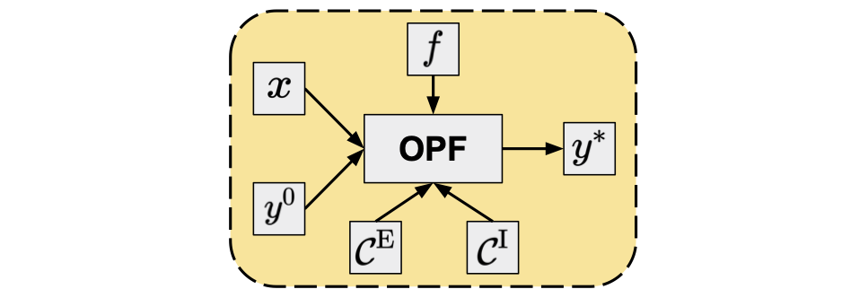 Figure 1. OPF as an operator.
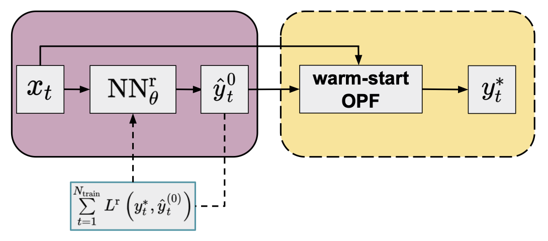 Figure 2. Flowchart of the warm-start method (yellow panel) in combination with an NN regressor (purple panel, default arguments of OPF operator are omitted for clarity) trained by minimizing a conventional loss function.
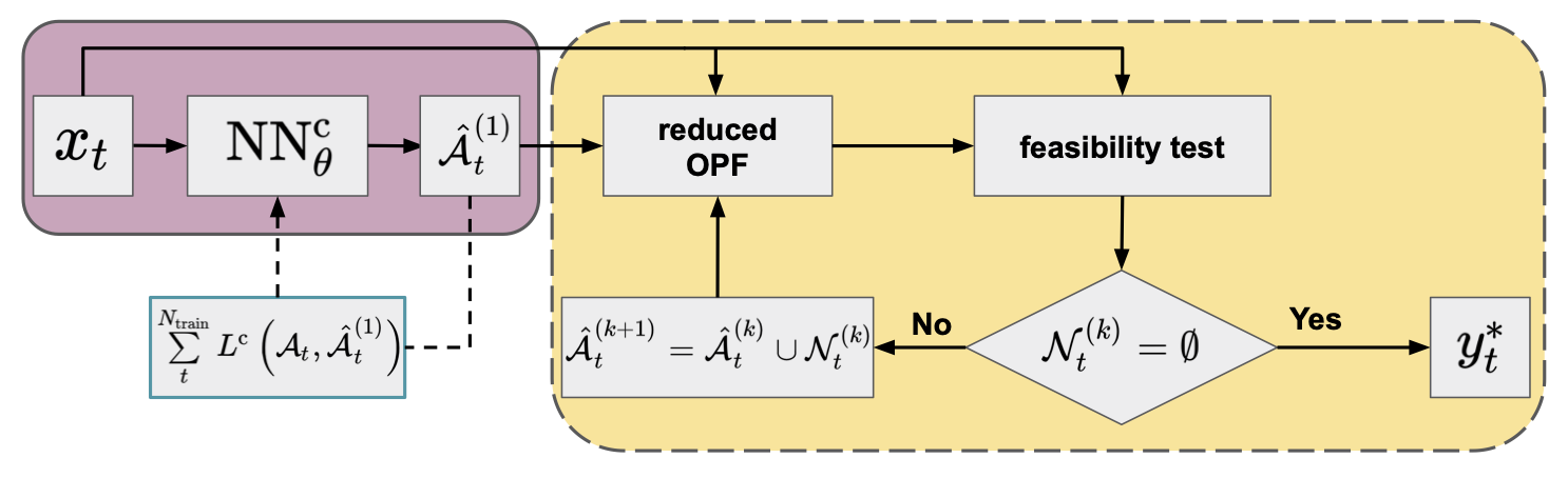 Figure 3. Flowchart of the iterative feasibility test method (yellow panel) in combination with a NN classifier (purple panel; default arguments of OPF operator are omitted for clarity) trained by minimizing a conventional loss function.
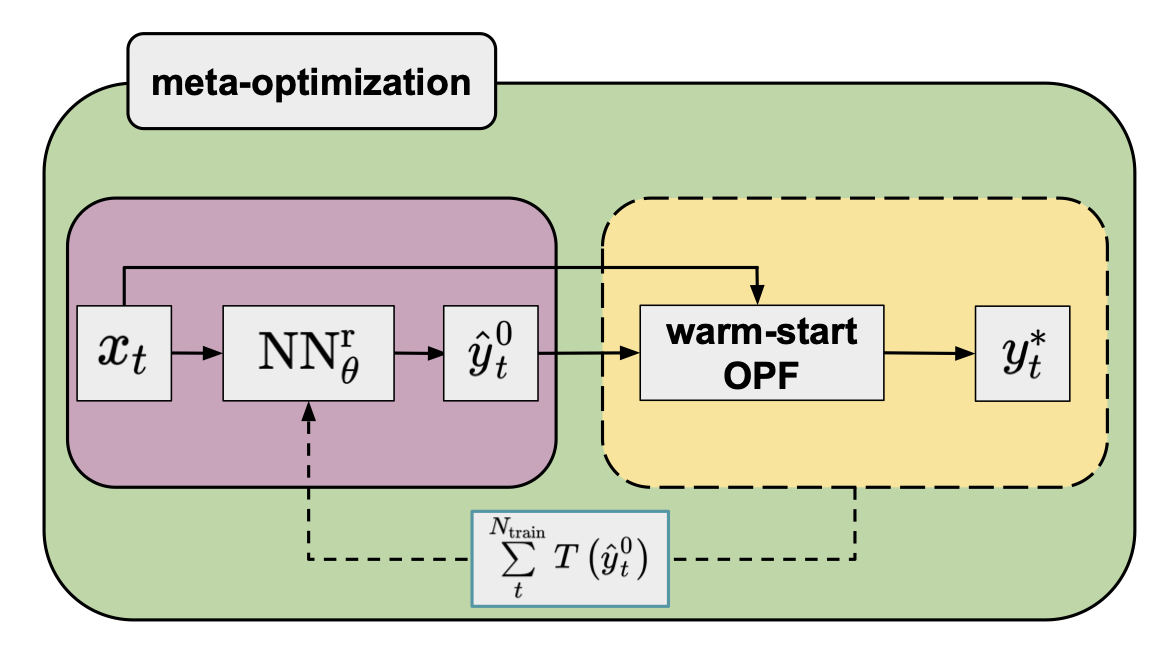 Figure 4. Flowchart of the warm-start method (yellow panel) in combination with an NN regressor (purple panel; default arguments of the OPF operator are omitted for clarity) trained by minimizing a meta-loss function that is a sum of the computational time of warm-started OPFs of the training data.
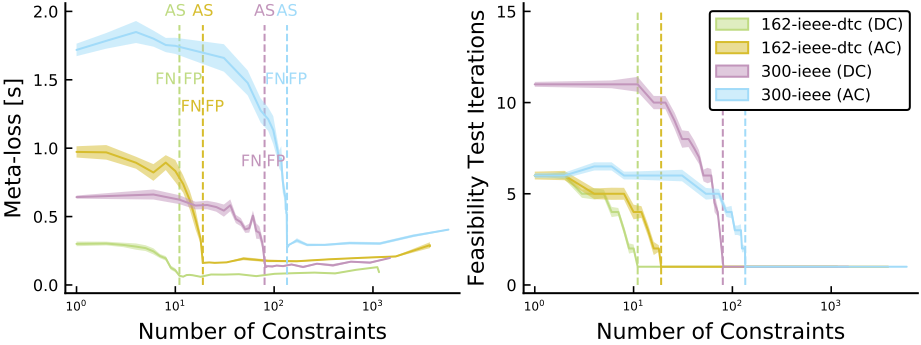 Figure 5. Profile of the meta-loss (total computational time) and number of iterations within the iterative feasibility test as functions of the number of constraints for two grids, and a comparison of DC vs. AC formulations. Perfect classifiers with the active set (AS) are indicated by vertical dashed lines, with the false positive (FP) region to the right, and the false negative (FN) region to the left.
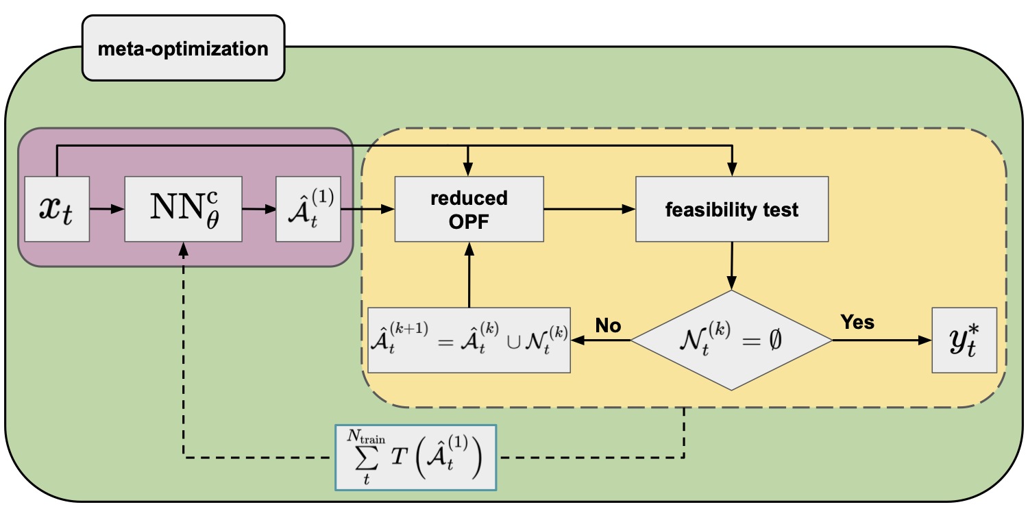 Figure 6. Flowchart of the iterative feasibility test method (yellow panel) in combination with an NN classifier (purple panel; default arguments of the OPF operator are omitted for clarity) trained by minimizing a meta-loss function that is a sum of the computational time of the iterative feasibility tests of the training data.
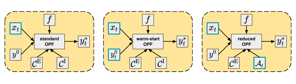 Figure 1. Main approaches to solving OPF. Varying arguments are highlighted, while other arguments are potentially fixed.
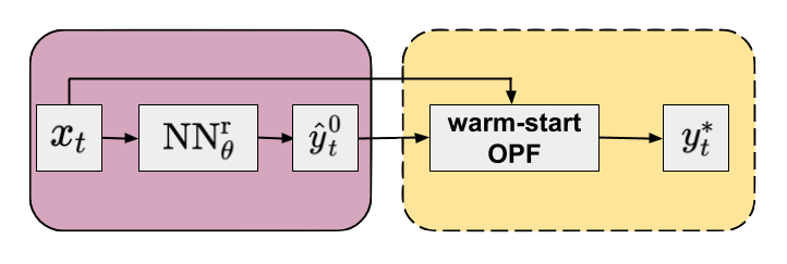 Figure 2. Flowchart of the warm-start method (yellow panel) in combination with an NN regressor (purple panel). Default arguments of OPF operator are omitted for clarity.
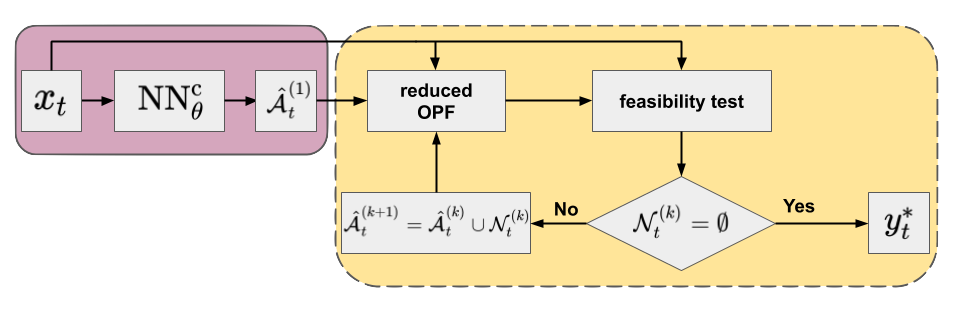 Figure 3. Flowchart of the iterative feasibility test method (yellow panel) in combination with an NN classifier (purple panel) Default arguments of OPF operator are omitted for clarity.