 Invenia Blog
Factor the Joint! Intoducing GPAR: a Multi-output GP Model
18 Dec 2018Introduction
Gaussian processes (GP) provide a powerful and popular approach to nonlinear single-output regression. Most regression problems, however, involve multiple outputs rather than a single one. When modelling such data, it is key to capture the dependencies between the outputs. For example, noise in the output space might be correlated, or, while one output might depend on the inputs in a complex (deterministic) way, it may depend quite simply on other output variables. In such cases a multi-output model is required. Let’s examine such an example.
A Multi-output Modelling Example
Consider the problem of modelling the world’s average CO2 level \(C(t)\), temperature \(T(t)\), and Arctic sea ice extent \(I(t)\) as a function of time \(t\). By the greenhouse effect, one can imagine that the temperature \(T(t)\) is a complicated stochastic function \(f_1\) of CO2 and time: \(T(t) = f_1(C(t),t)\). Similarly, the Arctic sea ice extent \(I(t)\) can be modelled as another complicated function \(f_2\) of temperature, CO2, and time: \(I(t) = f_2(T(t),C(t),t)\). These functional relationships are depicted in the figure below:
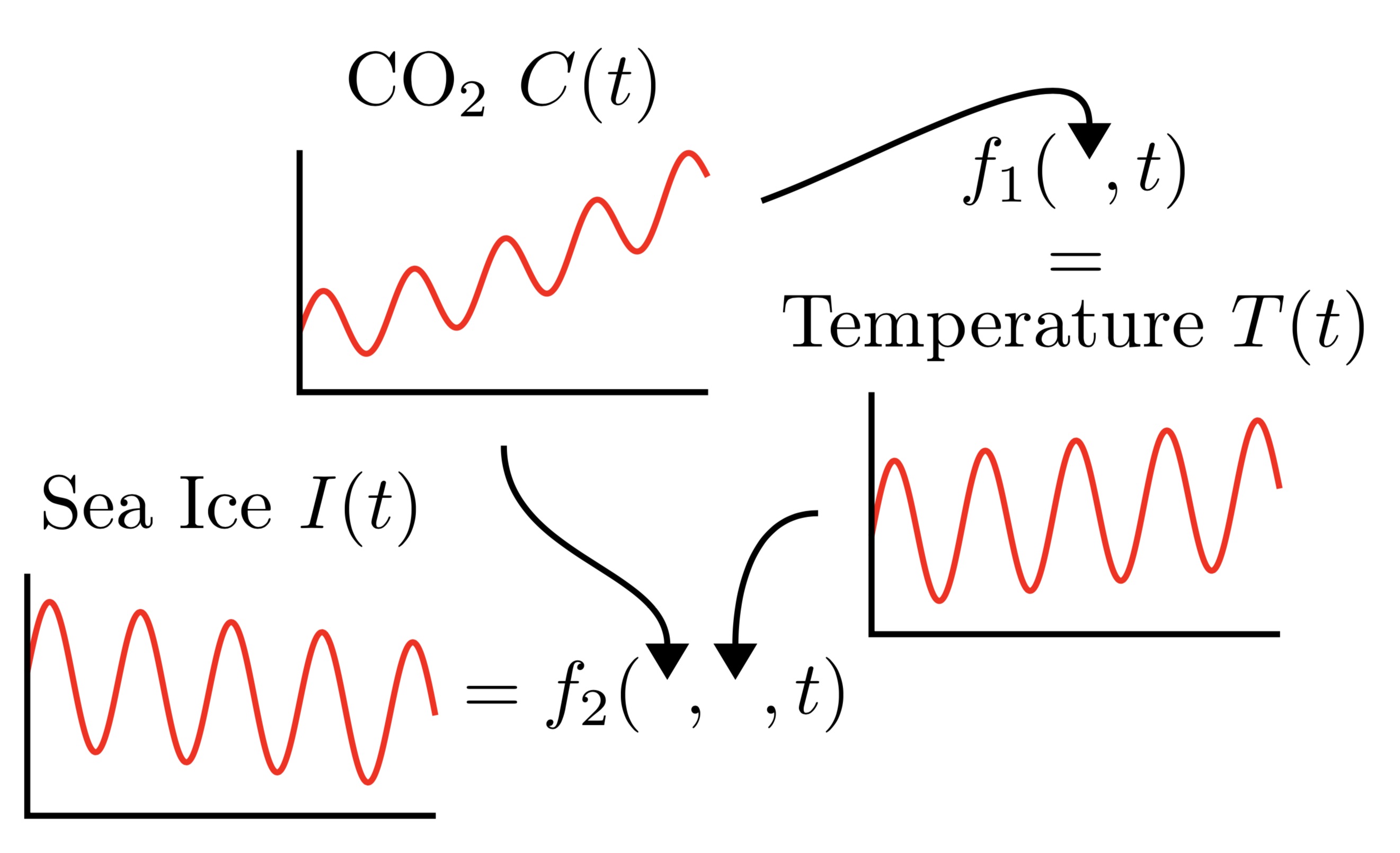
This structure motivates the following model where we have conditional probabilities modelling the underlying functions \(f_1\) and \(f_2\), and the full joint ditribution can be expressed as
\[p(I(t),T(t),C(t)) =p(C(t)) \underbrace{p(T(t)\cond C(t))}_{\text{models $f_1$}} \underbrace{p(I(t)\cond T(t), C(t))}_{\text{models $f_2$}}.\]More generally, consider the problem of modelling \(M\) outputs \(y_{1:M} (x) = (y1(x), . . . , yM (x))\) as a function of the input \(x\). Applying the product rule yields
\[p(y_{1:M}(x)) \label{eq:product_rule} =p(y_1(x)) \underbrace{p(y_2(x)\cond y_1(x))}_{\substack{\text{$y_2(x)$ as a random}\\ \text{function of $y_1(x)$}}} \;\cdots\; \underbrace{p(y_M(x)\cond y_{1:M-1}(x)),}_{\substack{\text{$y_M(x)$ as a random}\\ \text{function of $y_{1:M-1}(x)$}}}\]which states that \(y_1(x)\), like CO2, is first generated from \(x\) according to some unknown random function \(f_1\); that \(y_2(x)\), like temperature, is then generated from \(y_1(x)\) and \(x\) according to some unknown random function \(f_2\); that \(y_3(x)\), like the Arctic sea ice extent, is then generated from \(y_2(x)\), \(y_1(x)\), and \(x\) according to some unknown random function \(f_3\); et cetera:
\begin{align} y_1(x) &= f_1(x), & f_1 &\sim p(f_1), \newline y_2(x) &= f_2(y_1(x), x), & f_2 &\sim p(f_2), \newline y_3(x) &= f_3(y_{1:2}(x), x), & f_3 &\sim p(f_3), \newline &\;\vdots \nonumber \newline y_M(x) &= f_M(y_{1:M-1}(x),x) & f_M & \sim p(f_M). \end{align}
GPAR, the Gaussian Process Autoregressive Regression Model, models these unknown functions \(f_{1:M}\) with Gaussian Processes.
Modelling According to the Product Rule
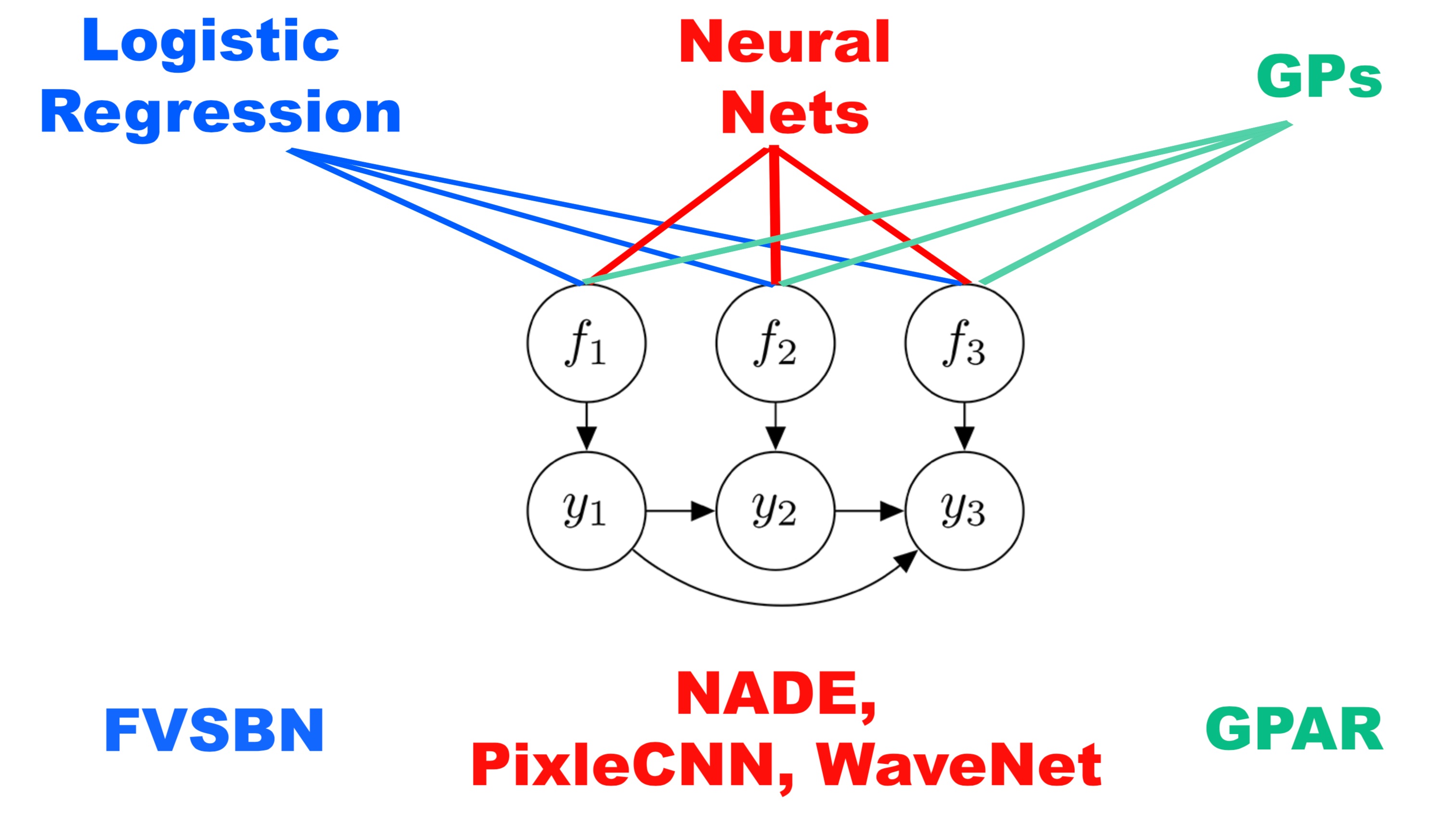
GPAR is not the first model to use the technique of factoring the joint distribution using the product rule and modelling each of the conditionals. A recognized advantage of this procedure is that if each of the individual conditional models is tractable then the entire model is also tractable. It also transforms the multi-output regression task into several single-output regression tasks which are easy to handle.
There are many interesting approaches to this problem, using various incarnations of neural networks. Neal [1992] and Frey et al. [1996] use logistic-regression-style models for the Fully Visible Sigmoid Belief Network (FVSBN), Larochelle and Murray [2011] use feed forward neural networks in NADE, and RNNs and convolutions are used in Wavenet (van den Oord et al., [2016]) and PixelCNN (van den Oord et al., [2016]).
In particular, if the observations are real-valued, a standard architecture lets the conditionals be Gaussian with means encoded by neural networks and fixed variances. Under broad conditions, if these neural networks are replaced by Bayesian neural networks with independent Gaussian priors over the weights, we recover GPAR as the width of the hidden layers goes to infinity (Neal, [1996]; Matthews et al., [2018]).
Other Multi-output GP Models
There are also many other multi-output GP models, many – but not all – of which consist of a “mixing” generative procedure: a number of latent GPs are drawn from GP priors and then “mixed” using a matrix multiplication, transforming the functions to the output space. Many of the GP based multi-output models are recoverable by GPAR, often in a much more tractable way. We discuss this further in our paper.
Some Issues With GPAR
Output Ordering
To construct GPAR, an ordering of outputs must be determined. We found that in many cases the ordering and the dependency structure of the outputs is obvious. If the order is not obvious, however, how can we choose one? We would like the ordering which maximizes the joint marginal likelihood of the entire GPAR model but, in most cases, building GPAR for all permutations of orderings is intractable. A more realistic approach would be to perform a greedy search: the first dimension would be determined by constructing a single output GP for each of the output dimensions and selecting the dimension that yields the largest marginal likelihood. The second dimension would then be selected by building a GP(AR) conditional on the first dimension and selecting the largest marginal likelihood, etc. In simple synthetic experiments, by permuting the generative ordering of observations, GPAR is able to recover the true ordering.
Missing Datapoints
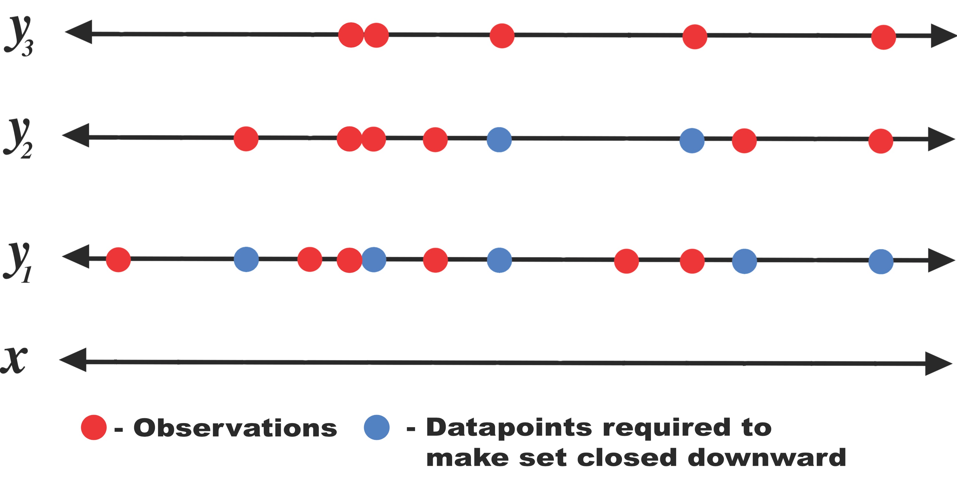
In order to use GPAR, the training dataset should be what we define to be “closed downward”: let \(D\) be a collection of observations of the form \((x, y_i)\) where \(y_i\) is observation in output dimension \(i\) at input location \(x\). \(D\) is closed downward if \((x, y_i) \in D\) implies that \((x, y_j) \in D\) for all \(j \leq i\).
This is not an issue if the dataset is complete, i.e., we have all output observations for each datapoint. However, in real-world cases some of the observations may be missing, resulting in datasets that are not closed downwards. In such cases, only certain orderings are allowed, or some parts of the dataset must be removed to construct one that is closed downwards. This could result in either a suboptimal model or in throwing away valuable information. To get around this issue, in our experiments we imputed missing values using the mean predicted by the previous conditional GP. The correct thing to do would be to sample from the previous conditional GP to integrate out the missing values, but in our experiments we found that simply using the mean works well.
What Can GPAR Do?
GPAR is well suited for problems where there is a strong functional relationship between outputs and for problems where observation noise is richly structured and input-dependent. To demonstrate this we tested GPAR on some synthetic problems.
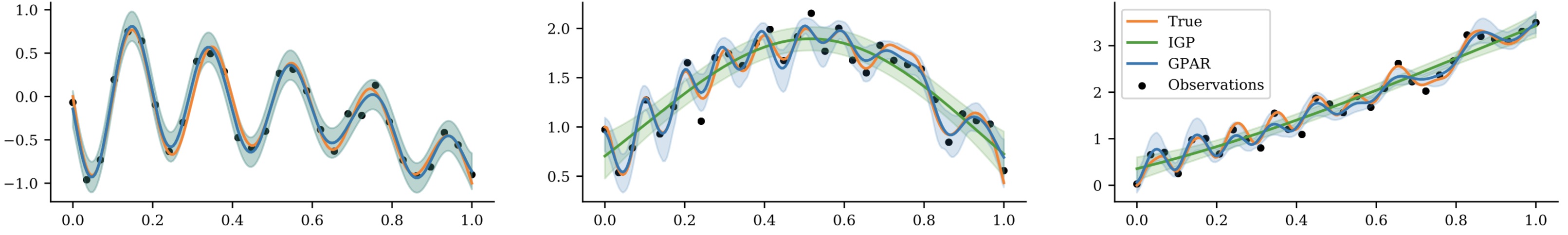
First, we test the ability to leverage strong functional relationships between the outputs. Consider three outputs \(y_1\), \(y_2\), and \(y_3\), which depend nonlinearly on each other:
\begin{align} y_1(x) &= -\sin(10\pi(x+1))/(2x + 1) - x^4 + \epsilon_1, \newline y_2(x) &= \cos^2(y_1(x)) + \sin(3x) + \epsilon_2, \newline y_3(x) &= y_2(x)y_1^2(x) + 3x + \epsilon_3, \end{align}
where \(\epsilon_1, \epsilon_2, \epsilon_3 {\sim} \mathcal{N}(0, 1)\). By substituting \(y_1\) and \(y_2\) into \(y_3\), we see that \(y_3\) can be expressed directly in terms of \(x\), but via a very complex function. This function of \(x\) is difficult to model with few data points. The dependence of \(y_3\) on \(y_1\) and \(y_2\) is much simpler. Therefore, as GPAR can exploit direct dependencies between \(y_{1:2}\) and \(y_3\), it should be presented with a simpler task compared to predicting \(y_3\) from \(x\) directly.
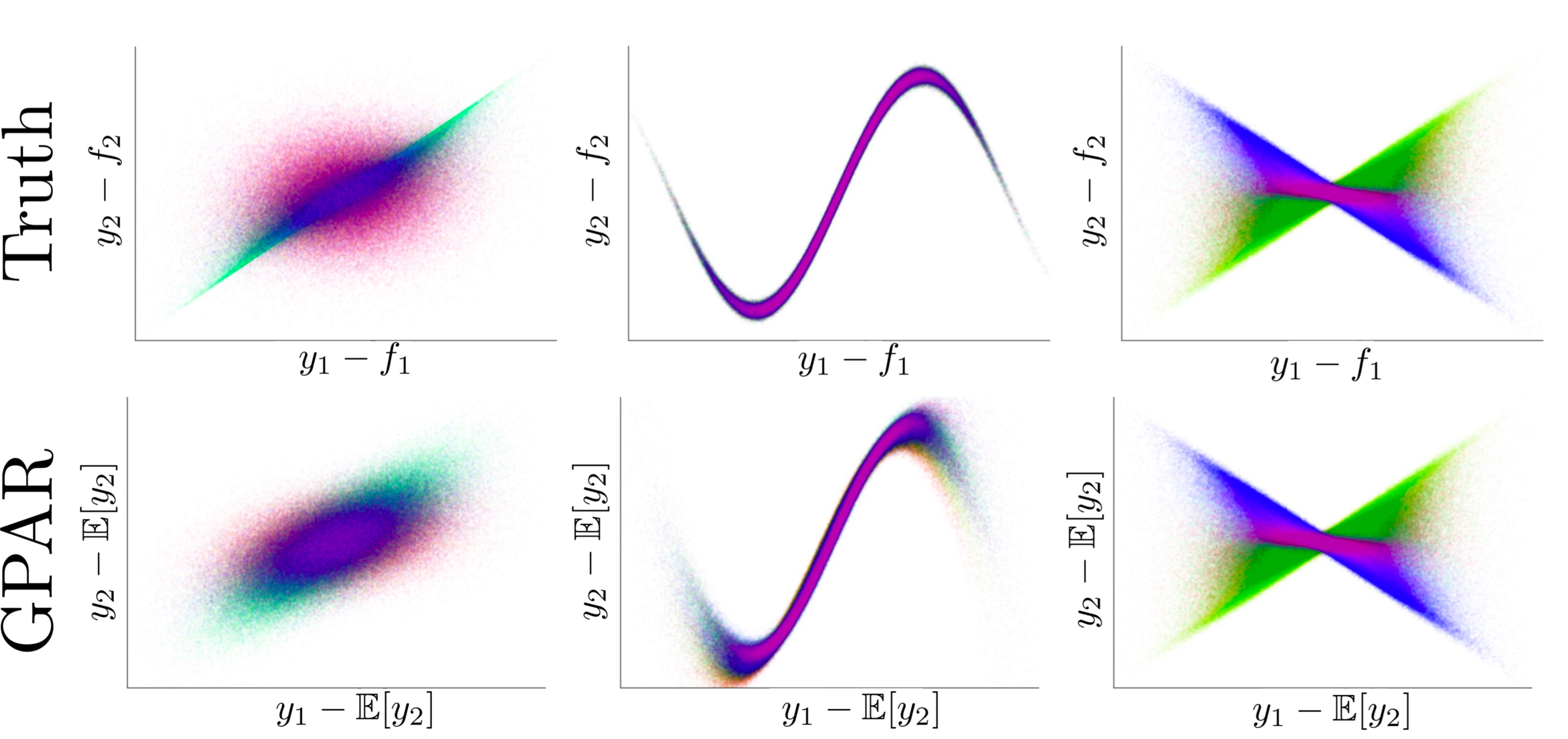
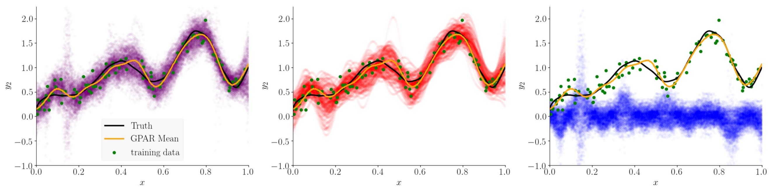
Second, we test GPAR’s ability to capture non-Gaussian and input-dependent noise. Consider the following three schemes in which two outputs are observed under various noise conditions: \(y_1(x) = f_1(x) + \epsilon_1\) and
\begin{align} \text{(1): } y_2(x) &= f_2(x) + \sin^2(2 \pi x)\epsilon_1 + \cos^2(2 \pi x) \epsilon_2, \newline \text{(2): } y_2(x) &= f_2(x) + \sin(\pi\epsilon_1) + \epsilon_2, \newline \text{(3): } y_2(x) &= f_2(x) + \sin(\pi x) \epsilon_1 + \epsilon_2, \end{align}
where \(\epsilon_1, \epsilon_2 \sim \mathcal{N}(0, 1)\), and \(f_1\) and \(f_2\) are nonlinear functions of \(x\):
\begin{align} f_1(x) &= -\sin(10\pi(x+1))/(2x + 1) - x^4 \newline f_2(x) &= \frac15 e^{2x}\left(\theta_{1}\cos(\theta_{2} \pi x) + \theta_{3}\cos(\theta_{4} \pi x) \right) + \sqrt{2x}, \end{align}
where the \(\theta\)s are constant values. All three schemes have i.i.d. homoscedastic Gaussian noise in \(y_1\) making \(y_1\) easy to learn for GPAR. The noise in \(y_2\) depends on that in \(y_1\), and can be heteroscedastic. The task for GPAR is to learn the scheme’s noise structure.
Note that we don’t have to make any spectial modelling assumptions to capture these noise structures: we still model the conditional distributions with GPs assuming i.i.d. Gaussian noise. We can now add components to our kernel composition to specifically model the structured noise. A figure below shows this decomposition.
Using the kernel decomposition it is possible to analyse both the functional and noise structure in an automated way similar to the work done by Duvenaud et al. in (Structure discovery in nonparametric regression through compositional kernel search, 2014).
Real World Benchmarks
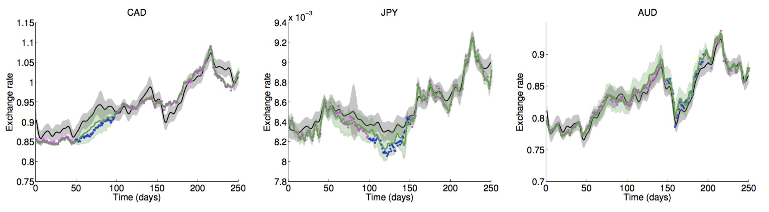
We compared GPAR to the state-of-the-art multi-output GP models on some standard benchmarks and showed that not only is GPAR often easier to implement and is faster than these methods, but it also yields better results. We tested GPAR on an EEG data set which consists of 256 voltage measurements from 7 electrodes placed on a subject’s scalp while the subject is shown a certain image; the Jura data set which comprises metal concentration measurements collected from the topsoil in a 14.5 square kilometer region of the Swiss Jura; and an exchange rates data set which consists of the daily exchange rate w.r.t. USD of the top ten international currencies (CAD, EUR, JPY, GBP, CHF,AUD, HKD, NZD, KRW, and MXN) and three preciousmetals (gold, silver, and platinum) in the year 2007. The plot below shows the comparison between GPAR and independent GPs:
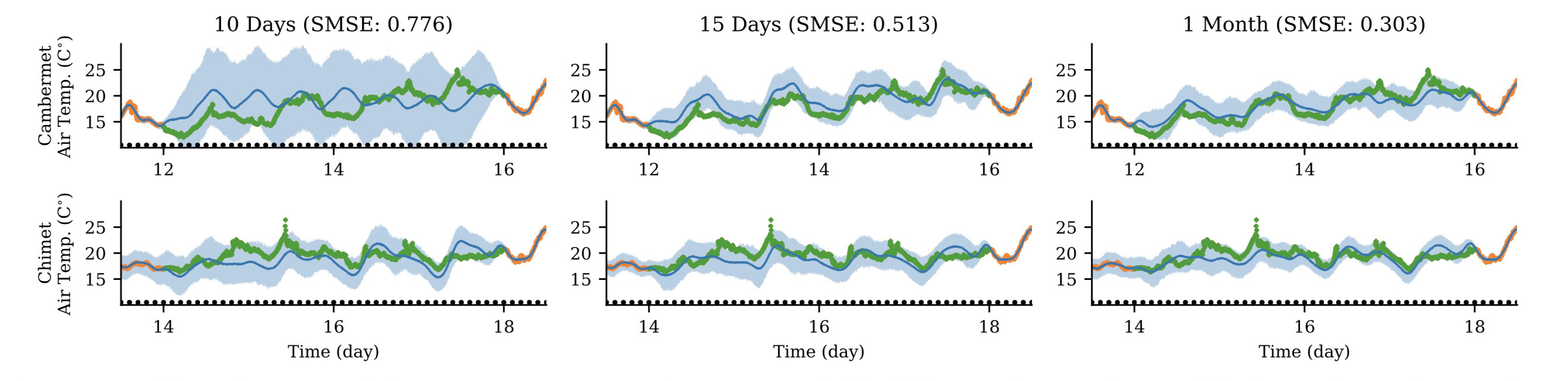
Lastly, a tidal height, wind speed, and air temperature data set (http://www.bramblemet.co.uk, http://cambermet.co.uk, http://www.chimet.co.uk, and http://sotonmet.co.uk) which was collected at 5 minute intervals by four weather stations: Bramblemet, Cambermet, Chimet, and Sotonmet, all located in Southampton, UK. The task in this last experiment is to predict the air temperature measured by Cambermet and Chimet from all other signals. Performance is measured with the SMSE. This experiment serves two purposes. First, it demonstrates that it is simple to scale GPAR to large datasets using off-the-shelf inducing point techniques for single-output GP regression. In our case, we used the variational inducing point method by Titsias (2009) with 10 inducing points per day. Second, it shows that scaling to large data sets enables GPAR to better learn dependencies between outputs, which, importantly, can significantly improve predictions in regions where outputs are partially observed. Using as training data 10 days (days [10,20), roughly 30k points), 15 days (days [18,23), roughly 47k points), and the whole of July (roughly 98k points), make predictions of 4 day periods of the air temperature measured by Cambermet and Chimet. Despite the additional observations not correlating with the test periods, we observe clear (though dimishining) improvements in the predictions as the training data is increased.
Future Directions
An exciting future application of GPAR is to use compositional kernel search (Lloyd et al., [2014]) to automatically learn and explain dependencies between outputs and inputs. Further insights into the structure of the data could be gained by decomposing GPAR’s posterior over additive kernel components (Duvenaud, [2014]). These two approaches could be developed into a useful tool for automatic structure discovery. Two further exciting future applications of GPAR are modelling of environmental phenomena and improving data efficiency of existing Bayesian optimisation tools (Snoek et al., [2012]).
References
- Duvenaud, D. (2014). Automatic Model Construction with Gaussian Processes. PhD thesis, Computational and Biological Learning Laboratory, University of Cambridge.
- Frey, B. J., Hinton, G. E., and Dayan, P. (1996). Does the wake-sleep algorithm produce good density estimators? In Advances in neural information processing systems, pages 661–667.
- Larochelle, H. and Murray, I. (2011). The neural autoregressive distribution estimator. In AISTATS, volume 1, page 2.
- Matthews, A. G. d. G., Rowland, M., Hron, J., Turner, R. E., and Ghahramani, Z. (2018). Gaussian process behaviour in wide deep neural networks. arXiv preprint arXiv:1804.11271.
- Lloyd, J. R., Duvenaud, D., Grosse, R., Tenenbaum, J. B., and Ghahramani, Z. (2014). Automatic construction and natural-language description of nonparametric regression models. In Association for the Advancement of Artificial Intelligence (AAAI).
- Neal, R. M. (1996). Bayesian learning for neural networks, volume 118. Springer Science & Business Media.
- Snoek, J., Larochelle, H., and Adams, R. P. (2012). Practical bayesian optimization of machine learning algorithms. In Advances in Neural Information Processing * Systems, pages 2951–2959.
- van den Oord, A., Kalchbrenner, N., Espeholt, L., Vinyals, O., Graves, A., et al. (2016). Conditional image generation with pixelcnn decoders. In Advances in Neural Information Processing Systems, pages 4790–4798.