Using Neural Networks for Predicting Solutions to Optimal Power Flow

11 Oct 2021

Author: Letif Mones

In a previous blog post, we discussed the fundamental concepts of optimal power flow (OPF), a core problem in operating electricity grids. In their principal form, AC-OPFs are non-linear and non-convex optimization problems that are in general expensive to solve. In practice, due to the large size of electricity grids and number of constraints, solving even the linearized approximation (DC-OPF) is a challenging optimization requiring significant computational effort. Adding to the difficulty, the growing integration of renewable generation has increased uncertainty in grid conditions and increasingly requires grid operators to solve OPF problems in near real-time. This has led to new research efforts in using machine learning (ML) approaches to shift the computational effort away from real-time (optimization) to offline training, potentially providing an almost instant prediction of the outputs of OPF problems.

This blog post focuses on a specific set of machine learning approaches that applies neural networks (NNs) to predict (directly or indirectly) solutions to OPF. In order to provide a concise and common framework for these approaches, we consider first the general mathematical form of OPF and the standard technique to solve it: the interior-point method. Then, we will see that this optimization problem can be viewed as an operator that maps a set of quantities to the optimal value of the optimization variables of the OPF. For the simplest case, when all arguments of the OPF operator are fixed except the grid parameters, we introduce the term, OPF function. We will show that all the NN-based approaches discussed here can be considered as estimators of either the OPF function or the OPF operator.¹

General form of OPF

OPF problems can be expressed in the following concise form of mathematical programming:

\[\begin{equation} \begin{aligned} & \min \limits_{y}\ f(x, y) \\ & \mathrm{s.\ t.} \ \ c_{i}^{\mathrm{E}}(x, y) = 0 \quad i = 1, \dots, n \\ & \quad \; \; \; \; \; c_{j}^{\mathrm{I}}(x, y) \ge 0 \quad j = 1, \dots, m \\ \end{aligned} \label{opt} \end{equation}\]

where \(x\) is the vector of grid parameters and \(y\) is the vector of optimization variables, \(f(x, y)\) is the objective (or cost) function to minimize, subject to equality constraints \(c_{i}^{\mathrm{E}}(x, y) \in \mathcal{C}^{\mathrm{E}}\) and inequality constraints \(c_{j}^{\mathrm{I}}(x, y) \in \mathcal{C}^{\mathrm{I}}\). For convenience we write \(\mathcal{C}^{\mathrm{E}}\) and \(\mathcal{C}^{\mathrm{I}}\) for the sets of equality and inequality constraints, respectively, with corresponding cardinalities \(n = \lvert \mathcal{C}^{\mathrm{E}} \rvert\) and \(m = \lvert \mathcal{C}^{\mathrm{I}} \rvert\). The objective function is optimized solely with respect to the optimization variables (\(y\)), while variables (\(x\)) parameterize the objective and constraint functions. For example, for a simple economic dispatch (ED) problem \(x\) includes voltage magnitudes and active powers of generators, \(y\) is a vector of active and reactive power components of loads, the objective function is the cost of the total real power generation, equality constraints include the power balance and power flow equations, while inequality constraints impose lower and upper bounds on other critical quantities.

The most widely used approach to solving the above optimization problem (that can be non-linear, non-convex and even mixed-integer) is the interior-point method.^{2 3 4} The interior-point (or barrier) method is a highly efficient iterative algorithm. However, it requires the computation of the Hessian (i.e. second derivatives) of the Lagrangian of the system with respect to the optimization variables at each iteration step. Due to the non-convex nature of the power flow equations appearing in the equality constraints, the method can be prohibitively slow for large-scale systems.

The formulation of eq. \(\eqref{opt}\) gives us the possibility of looking at OPF as an operator that maps the grid parameters (\(x\)) to the optimal value of the optimization variables (\(y^{*}\)). In a more general sense, the objective and constraint functions are also arguments of this operator. Also, in this discussion we assume that, if feasible, the exact solution of the OPF problem is always provided by the interior-point method. Therefore, the operator is parameterized implicitly by the starting value of the optimization variables (\(y^{0}\)). The actual value of \(y^{0}\) can significantly affect the convergence rate of the interior-point method and the total computational time, and for non-convex formulations (where multiple local minima might exist) even the optimal point can differ. The general form of the OPF operator can be written as:

\[\begin{equation} \Phi: \Omega \to \mathbb{R}^{n_{y}}: \quad \Phi\left( x, y^{0}, f, \mathcal{C}^{\mathrm{E}}, \mathcal{C}^{\mathrm{I}} \right) = y^{*}, \label{opf-operator} \end{equation}\]

where \(\Omega\) is an abstract set within the values of the operator arguments are allowed to change and \(n_{y}\) is the dimension of the optimization variables. We note that a special case of the general form is the DC-OPF operator, whose mathematical properties have been thoroughly investigated in a recent work.⁵

In many recurring problems, most of the arguments of the OPF operator are fixed and only (some of) the grid parameters vary. For these cases, we introduce a simpler notation, the OPF function:

\[\begin{equation} F_{\Phi}: \mathbb{R}^{n_{x}} \to \mathbb{R}^{n_{y}}: \quad F_{\Phi}(x) = y^{*}, \label{opf-function} \end{equation}\]

where \(n_{x}\) and \(n_{y}\) are the dimensions of grid parameter and optimization variables, respectively. We also denote the set of all feasible points of OPF as \(\mathcal{F}_{\Phi}\). The optimal value \(y^{*}\) is a member of the set \(\mathcal{F}_{\Phi}\) and in the case when the problem is infeasible, \(\mathcal{F}_{\Phi} = \emptyset\).

The daily task of electricity grid operators is to provide solutions for OPF, given constantly changing grid parameters \(x_{t}\). The standard OPF approach would be to compute \(F_{\Phi}(x_{t}) = y_{t}^{*}\) using some default values of the other arguments of \(\Phi\). However, in practice this is used rather rarely as usually additional information about the grid is also available that can be used to obtain the solution more efficiently. For instance, it is reasonable to assume that for similar grid parameter vectors the corresponding optimal points are also close to each other. If one of these problems is solved then its optimal point can be used as the starting value for the optimization variables of the other problem, which can then converge significantly faster compared to some default initial values. This strategy is called warm-start and might be useful for consecutive problems, i.e. \(\Phi \left( x_{t}, y_{t-1}^{*}, f, \mathcal{C}^{\mathrm{E}}, \mathcal{C}^{\mathrm{I}} \right) = y_{t}^{*}\). Another way to reduce the computational time of solving OPF is to reduce the problem size. The OPF solution is determined by the objective function and all binding constraints. However, at the optimal point, not all of the constraints are actually binding and there is a large number of non-binding inequality constraints that can be therefore removed from the mathematical problem without changing the optimal point, i.e. \(\Phi \left( x_{t}, y^{0}, f, \mathcal{C}^{\mathrm{E}}, \mathcal{A}_{t} \right) = y_{t}^{*}\), where \(\mathcal{A}_{t}\) is the set of all binding inequality constraints of the actual problem (equality constraints are always binding). This formulation is called reduced OPF and it is especially useful for DC-OPF problems. The three main approaches discussed are depicted in Figure 1.

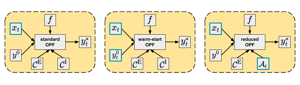Figure 1. Main approaches to solving OPF. Varying arguments are highlighted, while other arguments are potentially fixed.

NN-based approaches for predicting OPF solutions

The ML methods we will discuss apply either an estimator function (\(\hat{F}_{\Phi}(x_{t}) = \hat{y}_{t}^{*}\)) or an estimator operator (\(\hat{\Phi}(x_{t}) = \hat{y}_{t}^{*}\)) to provide a prediction of the optimal point of OPF based on the grid parameters.

We can categorize these methods in different ways. For instance, based on the estimator type they use, we can distinguish between end-to-end (aka direct) and hybrid (aka indirect) approaches. End-to-end methods use a NN as an estimator function and map the grid parameters directly to the optimal point of OPF. Hybrid or indirect methods apply an estimator operator that includes two steps: in the first step, a NN maps the grid parameters to some quantities, which are then used in the second step as inputs to some optimization problem resulting in the predicted (or even exact) optimal point of the original OPF problem.

We can also group techniques based on the NN predictor type: the NN can be used either as regressor or classifier.

Regression

The OPF function establishes a non-linear relationship between the grid parameters and optimization variables. In regression techniques, this complex relationship is approximated by NNs, treating the grid parameters as the input and the optimal values of the optimization variables as the output of the NN model.

End-to-end methods

End-to-end methods⁶ apply NNs as regressors, mapping the grid parameters (as inputs) directly to the optimal point of OPF (as outputs):

\[\begin{equation} \hat{F}_{\Phi}(x_{t}) = \mathrm{NN}_{\theta}^{\mathrm{r}}(x_{t}) = \hat{y}_{t}^{*}, \end{equation}\]

where the subscript \(\theta\) denotes all parameters (weights, biases, etc.) of the NN and the superscript \(\mathrm{r}\) indicates that the NN is used as a regressor. We note that once the prediction \(\hat{y}_{t}^{*}\) is computed, other dependent quantities (e.g. power flows) can be easily obtained by solving the power flow problem^{6 7} — given the prediction is a feasible point.

As OPF is a constrained optimization problem, the optimal point is not necessarily a smooth function of the grid parameters: changes of the binding status of constraints can lead to abrupt changes of the optimal solution. Also, the number of congestion regimes — i.e. the number of distinct sets of active (binding) constraints — increases exponentially with grid size. Therefore, in order to obtain sufficiently high coverage and accuracy of the model, a substantial amount of training data is required.

Warm-start methods

For real power grids, the available training data is rather limited compared to the system size. As a consequence, it is challenging to provide predictions by end-to-end methods that are optimal. Of even greater concern, there is no guarantee that the predicted optimal point is a feasible point (i.e. satisfies all constraints), and violation of important constraints could lead to severe security issues for the grid.

Nevertheless, the predicted optimal point can be utilized as a starting point to initialize an interior-point method. Interior-point methods (and actually most of the relevant optimization algorithms for OPF) can be started from a specific value of the optimization variables (warm-start optimization). The idea of the warm-start approaches is to use a hybrid model that first applies a NN for predicting a set-point, \(\hat{y}_{t}^{0} = \mathrm{NN}_{\theta}^{\mathrm{r}}(x_{t})\), from which a warm-start optimization can be performed.^{8 9} Using the previously introduced notation, we can write this approach as an estimator of the OPF operator, where the starting value of the optimization variables is estimated:

\[\begin{equation} \begin{aligned} \hat{\Phi}^{\mathrm{warm}}(x_{t}) & = \Phi \left( x_{t}, \hat{y}_{t}^{0}, f, \mathcal{C}^{\mathrm{E}}, \mathcal{C}^{\mathrm{I}} \right) \\ & = \Phi \left( x_{t}, \mathrm{NN}_{\theta}^{\mathrm{r}}(x_{t}), f, \mathcal{C}^{\mathrm{E}}, \mathcal{C}^{\mathrm{I}} \right) \\ &= y_{t}^{*} \quad . \end{aligned} \end{equation}\]

The flowchart of the approach is shown in Figure 2.

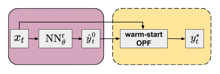Figure 2. Flowchart of the warm-start method (yellow panel) in combination with an NN regressor (purple panel). Default arguments of OPF operator are omitted for clarity.

It is important to note that warm-start methods provide an exact (locally) optimal point as it is eventually obtained from an optimization problem equivalent to the original one. Predicting an accurate set-point can significantly reduce the number of iterations (and so the computational cost) needed to obtain the optimal point compared to default heuristics of the optimization method.

Although the concept of warm-start interior-point techniques is quite attractive, there are some practical difficulties as well that we briefly discuss. First, because only primal variables are initialized, the duals still need to converge, as interior-point methods require a minimum number of iterations even if the primals are set to their optimal values. Trying to predict the duals with NN as well would make the task even more challenging. Second, if the initial values of primals are far from optimal (i.e. inaccurate prediction of set-points), the optimization can lead to a different local minimum. Finally, even if the predicted values are close to the optimal solution, as there are no guarantees on feasibility of the starting point, this could be located in a region resulting in substantially longer solve times or even convergence failure.

Classification

Predicting active sets

An alternative hybrid approach using an NN classifier (\(\mathrm{NN}_{\theta}^{\mathrm{c}}\)) leverages the observation that only a fraction of all constraints is actually binding at the optimum^{10 11}, so a reduced OPF problem can be formulated by keeping only the binding constraints. Since this reduced problem still has the same objective function as the original one, the solution should be equivalent to that of the original full problem: \(\Phi \left( x_{t}, y^{0}, f, \mathcal{C}^{\mathrm{E}}, \mathcal{A}_{t} \right) = \Phi \left( x_{t}, y^{0}, f, \mathcal{C}^{\mathrm{E}}, \mathcal{C}^{\mathrm{I}} \right) = y_{t}^{*}\), where \(\mathcal{A}_{t} \subseteq \mathcal{C}^{\mathrm{I}}\) is the active or binding subset of the inequality constraints (also note that \(\mathcal{C}^{\mathrm{E}} \cup \mathcal{A}_{t}\) contains all active constraints defining the specific congestion regime). This suggests a classification formulation, in which the grid parameters are used to predict the active set. The corresponding NN based estimator of the OPF operator can be written as:

\[\begin{equation} \begin{aligned} \hat{\Phi}^{\mathrm{red}}(x_{t}) &= \Phi \left( x_{t}, y^{0}, f, \mathcal{C}^{\mathrm{E}}, \hat{\mathcal{A}}_{t} \right) \\ &= \Phi \left( x_{t}, y^{0}, f, \mathcal{C}^{\mathrm{E}}, \mathrm{NN}_{\theta}^{\mathrm{c}}(x_{t}) \right) \\ &= \hat{y}_{t}^{*} \quad . \end{aligned} \end{equation}\]

Technically, the NN can be used in two ways to predict the active set. One approach is to identify all distinct active sets in the training data and train a multiclass classifier that maps the input to the corresponding active set.¹¹ Since the number of active sets increases exponentially with system size, for larger grids it might be better to predict the binding status of each non-trivial constraint by using a binary multi-label classifier.¹²

Iterative feasibility test

Imperfect prediction of the binding status of constraints (or active set) can lead to similar security issues as imperfect regression. This is especially important for false negative predictions, i.e. predicting an actually binding constraint as non-binding. As there may be violated constraints not included in the reduced model, one can use the iterative feasibility test to ensure convergence to an optimal point of the full problem.^{13 12} The procedure has been widely used by power grid operators. In combination with a classifier, it includes the following steps:

1. An initial active set of inequality constraints (\(\hat{\mathcal{A}}_{t}^{(1)}\)) is proposed by the classifier and a solution of the reduced problem is obtained.
2. In each feasibility iteration, \(k = 1, \ldots, K\), the optimal point of the actual reduced problem (\({\hat{y}_{t}^{*}}^{(k)}\)) is validated against the constraints \(\mathcal{C}^{\mathrm{I}}\) of the original full formulation.
3. At each step \(k\), the violated constraints \(\mathcal{N}_{t}^{(k)} \subseteq \mathcal{C}^{\mathrm{I}} \setminus \hat{\mathcal{A}}_{t}^{(k)}\) are added to the set of considered inequality constraints to form the active set of the next iteration: \(\hat{\mathcal{A}}_{t}^{(k+1)} = \hat{\mathcal{A}}_{t}^{(k)} \cup \mathcal{N}_{t}^{(k)}\).
4. The procedure is repeated until no violations are found (i.e. \(\mathcal{N}_{t}^{(k)} = \emptyset\)), and the optimal point satisfies all original constraints \(\mathcal{C}^{\mathrm{I}}\). At this point, we have found the optimal point to the full problem (\({\hat{y}_{t}^{*}}^{(k)} = y_{t}^{*}\)).

The flowchart of the iterative feasibility test in combination with NN is presented in Figure 3. As the reduced OPF is much cheaper to solve than the full problem, this procedure (if converged in few iterations) can be very efficient.

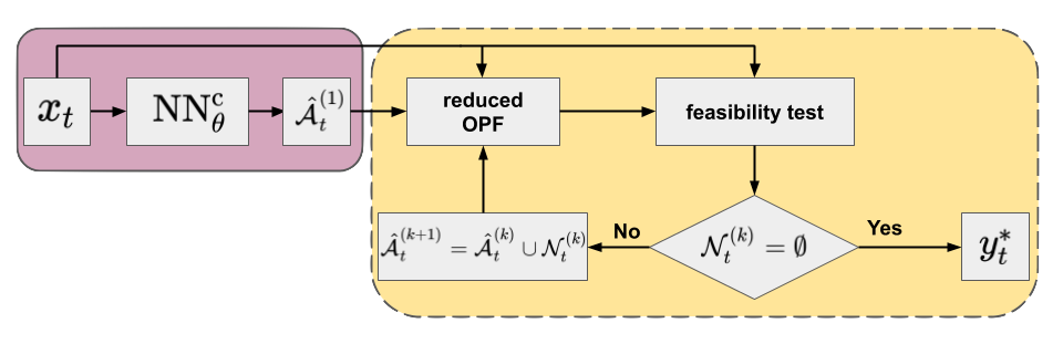Figure 3. Flowchart of the iterative feasibility test method (yellow panel) in combination with an NN classifier (purple panel) Default arguments of OPF operator are omitted for clarity.

Technical details of models

In this section, we provide a high level overview of the most general technical details used in the field.

Systems and samples

As discussed earlier, both the regression and classification approaches require a relatively large number of training samples, ranging between a few thousand and hundreds of thousands, depending on the OPF type, system size, and various grid parameters. Therefore, most of the works use synthetic grids of the Power Grid Library¹⁴ for which the generation of samples can be obtained straightforwardly. The size of the investigated systems usually varies between a few tens to a few thousands of buses and both DC- and AC-OPF problems can be investigated for economic dispatch, security constrained, unit commitment and even security constrained unit commitment problems. The input grid parameters are primarily the active and reactive power loads, although a much wider selection of varied grid parameters is also possible. The standard technique is to generate feasible samples by varying the grid parameters by a deviation of \(3-70\%\) from their default values and using multivariate uniform, normal, and truncated normal distributions.

Finally, we note that given the rapid increase of attention in the field it would be beneficial to have standard benchmark data sets in order to compare different models and approaches.¹²

Loss functions

For regression-based approaches, the most basic loss function optimized with respect to the NN parameters is the (mean) squared error. In order to reduce possible violations of certain constraints, an additional penalty term can be added to this loss function.

For classification-based methods, cross-entropy (multiclass classifier) or binary cross-entropy (multi-label classifier) functions can be applied with a possible regularization term.

NN architectures

Most of the models applied a fully connected NN (FCNN) from shallow to deep architectures. However, there are also attempts to take the grid topology into account, and convolutional (CNN) and graph (GNN) neural networks have been used for both regression and classification approaches. GNNs, which can use the graph of the grid explicitly, seemed particularly successful compared to FCNN and CNN architectures.¹⁵

Table 1. Comparison of some works using neural networks for predicting solutions to OPF. From each reference the largest investigated system is shown with corresponding number of buses (\(\lvert \mathcal{N} \rvert\)). Dataset size and grid input types are also presented. For sample generation \(\mathcal{U}\) and \(\mathcal{TN}\) denote uniform and truncated normal distributions, respectively and their arguments are the minimum and maximum factors multiplying the default grid parameter value. FCNN, CNN and GNN denote fully connected, convolutional and graph neural networks, respectively. SE, MSE and CE indicate squared error, mean squared error and cross-entropy loss functions, respectively, and cvpt denotes constraint violation penalty term.

Ref.	OPF	System	\(\lvert \mathcal{N} \rvert\)	Dataset	Input	Sampling	NN	Predictor	Loss
6	AC-ED	118-ieee	118	813k	loads	\(\mathcal{U}(0.9, 1.1)\)	FCNN	regressor	MSE + cvpt
16	AC-ED	300-ieee	300	236k	loads	\(\mathcal{U}(0.8, 1.2)\)	FCNN	regressor	SE + cvpt
7	AC-ED	118-ieee	118	100k	loads	\(\mathcal{TN}(0.3, 1.7)\) \(\mathcal{U}(0.8, 1.0)\)	FCNN	regressor	MSE
17	DC-SCED	300-ieee	300	55k	load	\(\mathcal{U}(0.9, 1.1)\)	FCNN	regressor	MSE + cvpt
18	AC-ED	118-ieee	118	13k	loads	\(\mathcal{U}(0.9, 1.1)\)	FCNN GNN	regressor	MSE
11	DC-ED	24-ieee-rts	24	50k	load	\(\mathcal{U}(0.97, 1.03)\)	FCNN	classifier	CE
19	AC-ED	France-Lyon	3411	10k	loads	\(\mathcal{U}(0.8, 1.2)\)	FCNN	regressor	SE + cvpt
20	AC-ED	30-ieee	30	12k	loads	\(\mathcal{U}(0.8, 1.2)\)	FCNN	regressor	SE + cvpt
21	DC-ED	300-ieee	300	100k	load	\(\mathcal{U}(0.4, 1.0)\)	FCNN	regressor	MSE
12	DC-ED	1354-pegase	1354	10k	load + 3 other params	\(\mathcal{U}(0.85, 1.15)\) \(\mathcal{U}(0.9, 1.1)\)	FCNN	classifier	CE
12	AC-ED	300-ieee	300	1k	loads + 5 other params	\(\mathcal{U}(0.85, 1.15)\) \(\mathcal{U}(0.9, 1.1)\)	FCNN	classifier	CE
15	AC-ED	300-ieee	300	10k	loads + 5 other params	\(\mathcal{U}(0.85, 1.15)\) \(\mathcal{U}(0.9, 1.1)\)	FCNN CNN GNN	regressor classifier	MSE CE
1	AC-ED	2853-sdet	2853	10k	loads	\(\mathcal{U}(0.8, 1.2)\)	FCNN CNN GNN	regressor classifier	MSE CE

Conclusions

By moving the computational effort to offline training, machine learning techniques to predict OPF solutions have become an intense research direction.

Neural network based approaches are particularly promising as they can effectively model complex non-linear relationships between grid parameters and generator set-points in electrical grids.

End-to-end approaches, which try to map the grid parameters directly to the optimal value of the optimization variables, can provide the most computational gain. However, they require a large training data set in order to achieve sufficient predictive accuracy, otherwise the predictions will not likely be optimal or even feasible.

Hybrid techniques apply a combination of an NN model and a subsequent OPF step. The NN model can be used to predict a good starting point for warm-starting the OPF, or to generate a series of efficiently reduced OPF models using the iterative feasibility test. Hybrid methods can, therefore, improve the efficiency of OPF computations without sacrificing feasibility and optimality. Neural networks of the hybrid models can be trained by using conventional loss functions that measure some form of the prediction error. In a subsequent blog post, we will show that compared to these traditional loss functions, a significant improvement of the computational gain of hybrid models can be made by optimizing the computational cost directly.

---