Memristive dynamics: a heuristic optimization tool

Author: Ana Zegarac and Francesco Caravelli

Introduction

In this post we will explore an interesting area of modern circuit theory and computing: how exotic properties of certain nanoscale circuit components (analogous to tungsten filament lightblulbs) can be used for solving certain optimization problems. Let’s start with a simple example: imagine a circuit made up of resistors, all of which have the same resistance.

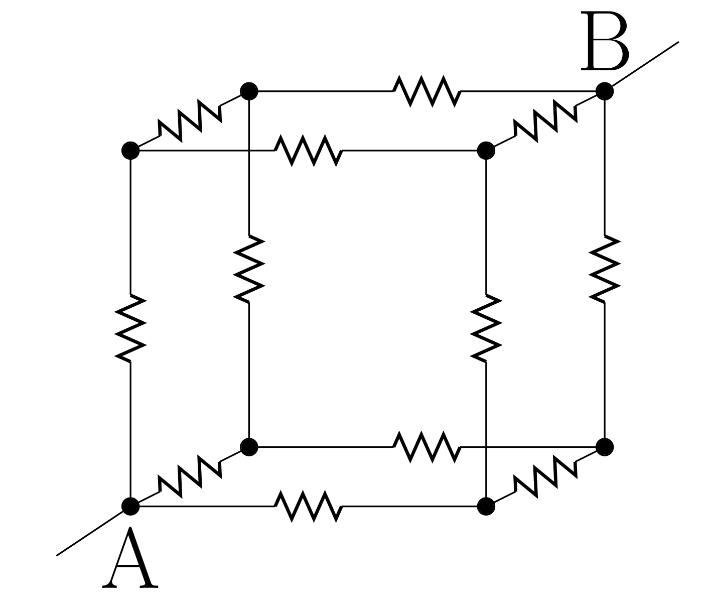
If we connect points A and B of the circuit above to a battery, current will flow through the conductors (let’s say from A to B), according to Kirchhoff’s laws. Because of the symmetry of the problem, the current splits at each intersection according to the inverse resistance rule, and so the currents will flow equally in all directions to reach B. This implies that if we follow the maximal current at each intersection, we can use this circuit to solve the minimum distance (or cost) problem on a graph. This can be seen as an example of a physical system performing analog computation. More generally, there is a deep connection between graph theory and resistor networks.

In 2008, researchers from Hewlett Packard introduced what is now called the “nanoscale memristor” ¹. This is a type of resistor made of certain metal oxides such as tungsten or titanium, for which the resistance changes as a function of time in a peculiar way. For the case of titanium dioxide, the resistance changes between two limiting values according to a simple convex law depending on an internal parameter, $w$, which is constrained between $0$ and $1$:

where,

and $I$ is the current in the device. This is a simple prototypical model of a memory-resistor, or memristor.

In the general case of a network of memristors, the above differential equation becomes ^{2 3 4 5}:

where $\mathrm{\Omega }$ is a matrix representing the circuit topology, $\overrightarrow{S}(t)$ are the applied voltages, and $W$ a diagonal matrix of the values of $w$ for each memristor in the network.

It is interesting to note that the equation above is related to a class of optimization problems, similarly to the case of a circuit of simple resistors. In the memristor case, this class is called quadratically unconstrained binary optimization (QUBO). The solution of a QUBO problem is the set of binary parameters, $w_i$, that minimize (or maximize) a function of the form:

This is because the dynamics of memristors, which are described by the equation above, is such that a QUBO functional is minimized. For the case of realistic circuits, $\mathrm{\Omega }$ satisfies certain properties which we will discuss below, but from the point of view of optimization theory, the system of differential equations can in principle be simulated for arbitrary $\mathrm{\Omega }$. Therefore, the memristive differential equation can serve as a heuristic solution method for an NP-Complete problem such as QUBO ⁴. These problems are NP-Complete because there is no known algorithm that is better than exhaustive search: because of the binary nature of the variables, in the worst case we have to explore all $2^N$ possible values of the variables $w$ to find the extrema of the problem. In a sense, the memristive differential equation is a relaxation of the QUBO problem to continuous variables.

Let’s look at an application to a standard problem: given the expected returns and covariance matrix between prices of some financial assets, which assets should an investor allocate capital to? This setup, with binary decision variables, is different than the typical question of portfolio allocation, in which the decision variables are real valued (fractions of wealth to allocate to assets). This is a combinatorial decision whether or not to invest in a given asset, but not the amount: the combinatorial Markowitz problem. The heuristic solution we propose has been introduced in the appendix of this paper. This can also be used as a screening procedure before the real portfolio optimization is performed, i.e., as a dimensionality reduction technique. More formally, the objective is to maximize:

where $r_i$ are the expected returns and $\mathrm{\Sigma }$ the covariance matrix. The mapping between the above and the equivalent memristive equation is given by:

The solution vector $S$ is obtained through inversion of the matrix $\mathrm{\Sigma }$ (if it is invertible). There are some conditions for this method to be suitable for heuristic optimization (related to the spectral properties of the matrix $J$), but as a heuristic method, this is much cheaper than exhaustive search: it requires a single matrix inversion which scales as $O(N^3)$, and the simulation of a first order differential equation which also requires a matrix inversion step by step, and thus scales as $O(T\cdot N^3)$ where $T$ is the number of time steps. We propose two approaches to this problem: one based on the most common Metropolis-Hasting-type algorithm (at each time step we flip a single weight, which can be referred as “Gibbs sampling”), and the other on the heuristic memristive equation.

Sample implementation

Below we include julia code for both algorithms.

using FillArrays
using LinearAlgebra

"""
    monte_carlo(
        expected_returns::Vector{Float64},
        Σ::Matrix{Float64},
        p::Float64,
        weights_init::Vector{Bool};
        λ::Float64=0.999995,
        effective_its::Int=3000,
        τ::Real=0.75,
    )

Execute Monte Carlo in order to find the optimal portfolio composition,
considering an asset covariance matrix `Σ` and a risk parameter `p`. `reg`
represents the regularisation constant for `Σ`, `λ` is the annealing factor, with
the temperature `τ` decreases at each step and `effective_its` determines how
many times, on average, each asset will have its weight changed.
"""
function monte_carlo(
    expected_returns::Vector{Float64},
    Σ::Matrix{Float64},
    p::Float64,
    weights_init::Vector{Bool};
    λ::Float64=0.999995,
    effective_its::Int=3000,
    τ::Real=0.75,
)
    weights = weights_init
    n = size(weights_init, 1)

    total_time = effective_its * n
    energies = Vector{Float64}(undef, total_time)

    # Compute energy of initial configuration
    energy_min = energy(expected_returns, Σ, p, weights_init)

    for t in 1:total_time
        # Anneal temperature
        τ = τ * λ
        # Randomly draw asset
        rand_index = rand(1:n)
        weights_current = weights
        # Flip weight from 0 to 1 and vice-versa
        weights_current[rand_index] = 1 - weights_current[rand_index]
        # Compute new energy
        energy_current = energy(expected_returns, Σ, p, weights)

        # Compute Boltzmann factor
        β = exp(-(energy_current - energy_min) / τ)

        # Randomly accept update
        if rand() < min(1, β)
            energy_min = energy_current
            weights = weights_current
        end

        # Store current best energy
        energies[t] = energy_min
    end
    return weights, energies
end

"""
    memristive_opt(
        expected_returns::Vector{Float64},
        Σ::Matrix{Float64},
        p::Float64,
        weights_init::Vector{<:Real};
        α=0.1,
        β=10,
        δt=0.1,
        total_time=3000,
    )

Execute optimisation via the heuristic "memristive" equation in order to find the
optimal portfolio composition, considering an asset covariance matrix `Σ` and a
risk parameter `p`. `reg` represents the regularisation constant for `Σ`, `α` and
`β` parametrise the memristor state (see Equation (2)),
`δt` is the size of the time step for the dynamical updates and `total_time` is
the number of time steps for which the dynamics will be run.
"""
function memristive_opt(
    expected_returns::Vector{Float64},
    Σ::Matrix{Float64},
    p::Float64,
    weights_init::Vector{<:Real};
    α=0.1,
    β=10,
    δt=0.1,
    total_time=3000,
)
    n = size(weights_init, 1)

    weights_series = Matrix{Float64}(undef, n, total_time)
    weights_series[:, 1] = weights_init
    energies = Vector{Float64}(undef, total_time)
    energies[1] = energy(expected_returns, Σ, p, weights_series[:, 1])

    # Compute resistance change ratio
    ξ = p / 2α
    # Compute Σ times applied voltages matrix
    ΣS = β * (α/2 * ones(n, 1) + (p/2 + α * ξ/3) * diag(Σ) - expected_returns)

    for t in 1:total_time-1
        update = δt * (α * weights_series[:, t] - 1/β * (Eye(n) + ξ *
            Σ * Diagonal(weights_series[:, t])) \ ΣS)
        weights_series[:, t+1] = weights_series[:, t] + update

        weights_series[weights_series[:, t+1] .> 1, t+1] .= 1.0
        weights_series[weights_series[:, t+1] .< 1, t+1] .= 0.0

        energies[t + 1] = energy(expected_returns, Σ, p, weights_series[:, t+1])
    end

    weights_final = weights_series[:, end]

    return weights_final, energies
end

"""
    energy(
        expected_returns::Vector{Float64},
        Σ::Matrix{Float64},
        p::Float64,
        weights::Vector{Float64},
    )

Return minus the expected return corrected by the variance of the portfolio,
according to the Markowitz approach. `Σ` represents the covariance of the assets,
`p` controls the risk tolerance and `weights` represent the (here binary)
portfolio composition.
"""
function energy(
    expected_returns::Vector{Float64},
    Σ::Matrix{Float64},
    p::Float64,
    weights::Vector{<:Real},
)
    -dot(expected_returns, weights) + p/2 * weights' * Σ * weights
end

A simple comparison between the two approaches shows the superiority of the memristor equation-based approach for this problem. We used a portfolio of 200 assets, with randomly generated initial allocations, expected returns and covariances. After 3000 effective iterations (that is 3000 times 200, the number of assets), the Monte Carlo approach leads to a corrected expected portfolio return of 3.9, while the memristive approach, in only a few steps, already converges to a solution with a corrected expected portfolio return of 19.5! Moreover, the solution found via Monte Carlo allocated investment to 91 different assets, while the memristor-based one only invested in 71 assets, thus showing an even better return to investment. There are obvious caveats here, as each of these methods have their own parameters which can be tuned in order to improve performance (which we did try doing), and it is known that Monte Carlo methods are ill-suited to combinatorial problems. Yet, such a stark difference shows how powerful memristors can be for optimization purposes (in particular for quickly generating some sufficiently good but not necessarily optimal solutions).

The equation for memristors is also interesting in other ways, for example, it has graph theoretical underpinnings ^{2 3 4}. Further, the memristor network equation is connected to optimization ^{5 6 7}. These are summarized in ⁸. For a general overview of the field of memristors, see the recent review ⁹.