A Gentle Introduction to Power Flow

04 Dec 2020

Author: Letif Mones

Although governed by simple physical laws, power grids are among the most complex human-made systems. The main source of the complexity is the large number of components of the power systems that interact with each other: one needs to maintain a balance between power injections and withdrawals while satisfying certain physical, economic, and environmental conditions. For instance, a central task of daily planning and operations of electricity grid operators¹ is to dispatch generation in order to meet demand at minimum cost, while respecting reliability and security constraints. These tasks require solving a challenging constrained optimization problem, often referred to as some form of optimal power flow (OPF).²

In a series of two blog posts, we are going to discuss the basics of power flow and optimal power flow problems. In this first post, we focus on the most important component of OPF: the power flow (PF) equations. For this, first we introduce some basic definitions of power grids and AC circuits, then we define the power flow problem.

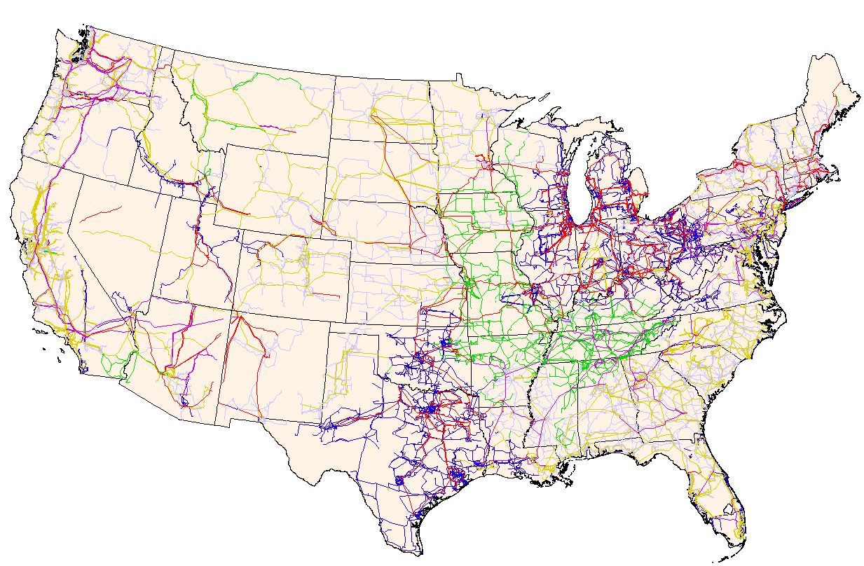Figure 1. Complexity of electricity grids: the electric power transmission grid of the United States (source: FEMA and Wikipedia).

Power grids as graphs

Power grids are networks that include two main components: buses that represent important locations of the grid (e.g. generation points, load points, substations) and transmission (or distribution) lines that connect these buses. It is pretty straightforward, therefore, to look at power grid networks as graphs: buses and transmission lines can be represented by nodes and edges of a corresponding graph. There are two equivalent graph models that can be used to derive the basic power flow equations³:

• directed graph representation (left panel of Figure 2): \(\mathbb{G}_{D}(\mathcal{N}, \mathcal{E})\);
• undirected graph representation (right panel of Figure 2): \(\mathbb{G}_{U}(\mathcal{N}, \mathcal{E} \cup \mathcal{E}^{R})\),

where \(\mathcal{N}\), \(\mathcal{E} \subseteq \mathcal{N} \times \mathcal{N}\) and \(\mathcal{E}^{R} \subseteq \mathcal{N} \times \mathcal{N}\) denote the set of nodes (buses), and the forward and reverse orientations of directed edges (branches) of the graph, respectively.

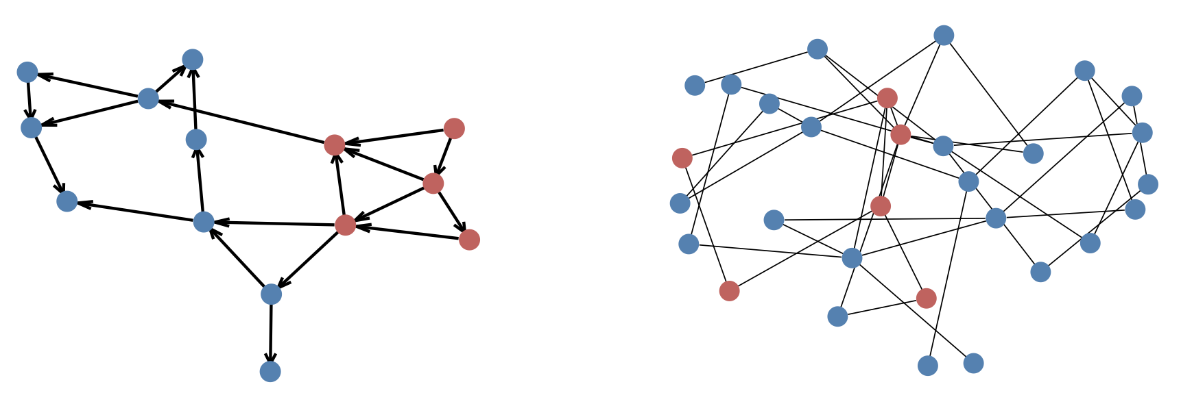Figure 2. Directed graph representation of synthetic grid 14-ieee (left) and undirected graph representation of synthetic grid 30-ieee (right). Red and blue circles denote generator and load buses, respectively.

Complex power in AC circuits

Power can be transmitted more efficiently at high voltages as high voltage (or equivalently, low current) reduces the loss of power due to its dissipation on transmission lines. Power grids generally use alternating current (AC) since the AC voltage can be altered (from high to low) easily via transformers. Therefore, we start with some notation and definitions for AC circuits.

The most important characteristics of AC circuits is that, unlike in direct current (DC) circuits, the currents and voltages are not constant in time: both their magnitude and direction vary periodically. Because of several technical reasons (like low losses and disturbances), power generators use sinusoidal alternating quantities that can be straightforwardly modeled by complex numbers.

We will consistently use capital and small letters to denote complex and real-valued quantities, respectively. For instance, let us consider two buses, \(i, j \in \mathcal{N}\), that are directly connected by a transmission line \((i, j) \in \mathcal{E}\). The complex power flowing from bus \(i\) to bus \(j\) is denoted by \(S_{ij}\) and it can be decomposed into its active (\(p_{ij}\)) and reactive (\(q_{ij}\)) components:

\[\begin{equation} S_{ij} = p_{ij} + \mathrm{j}q_{ij}, \end{equation}\]

where \(\mathrm{j} = \sqrt{-1}\). The complex power flow can be expressed as the product of the complex voltage at bus \(i\), \(V_{i}\) and the complex conjugate of the current flowing between the buses, \(I_{ij}^{*}\):

\[\begin{equation} S_{ij} = V_{i}I_{ij}^{*}, \label{power_flow} \end{equation}\]

It is well known that transmission lines have power losses due to their resistance (\(r_{ij}\)), which is a measure of the opposition to the flow of the current. For AC-circuits, a dynamic effect caused by the line reactance (\(x_{ij}\)) also plays a role. Unlike resistance, reactance does not cause any loss of power but has a delayed effect by storing and later returning power to the circuit. The effect of resistance and reactance together can be represented by a single complex quantity, the impedance: \(Z_{ij} = r_{ij} + \mathrm{j}x_{ij}\). Another useful complex quantity is the admittance, which is the reciprocal of the impedance: \(Y_{ij} = \frac{1}{Z_{ij}}\). Similarly to the impedance, the admittance can be also decomposed into its real, conductance (\(g_{ij}\)), and imaginary, susceptance (\(b_{ij}\)), components: \(Y_{ij} = g_{ij} + \mathrm{j}b_{ij}\).

Therefore, the current can be written as a function of the line voltage drop and the admittance between the two buses, which is an alternative form of Ohm’s law:

\[\begin{equation} I_{ij} = Y_{ij}(V_{i} - V_{j}). \end{equation}\]

Replacing the above expression for the current in the power flow equation (eq. \(\eqref{power_flow}\)), we get

\[\begin{equation} S_{ij} = Y_{ij}^{*}V_{i}V_{i}^{*} - Y_{ij}^{*}V_{i}V_{j}^{*} = Y_{ij}^{*} \left( |V_{i}|^{2} - V_{i}V_{j}^{*} \right). \end{equation}\]

The above power flow equation can be expressed by using the polar form of voltage, i.e. \(V_{i} = v_{i}e^{\mathrm{j} \delta_{i}} = v_{i}(\cos\delta_{i} + \mathrm{j}\sin\delta_{i})\) (where \(v_{i}\) and \(\delta_{i}\) are the voltage magnitude and angle of bus \(i\), respectively), and the admittance components:

\[\begin{equation} S_{ij} = \left(g_{ij} - \mathrm{j}b_{ij}\right) \left(v_{i}^{2} - v_{i}v_{j}\left(\cos\delta_{ij} + \mathrm{j}\sin\delta_{ij}\right)\right), \end{equation}\]

where for brevity we introduced the voltage angle difference \(\delta_{ij} = \delta_{i} - \delta_{j}\). Similarly, using a simple algebraic identity of \(g_{ij} - \mathrm{j}b_{ij} = \frac{g_{ij}^{2} + b_{ij}^{2}}{g_{ij} + \mathrm{j}b_{ij}} = \frac{|Y_{ij}|^{2}}{Y_{ij}} = \frac{Z_{ij}}{|Z_{ij}|^{2}} = \frac{r_{ij} + \mathrm{j}x_{ij}}{r_{ij}^{2} + x_{ij}^{2}}\), the impedance components-based expression has the following form:

\[\begin{equation} S_{ij} = \frac{r_{ij} + \mathrm{j}x_{ij}}{r_{ij}^{2} + x_{ij}^{2}} \left( v_{i}^{2} - v_{i}v_{j}\left(\cos\delta_{ij} + \mathrm{j}\sin\delta_{ij}\right)\right). \end{equation}\]

Finally, the corresponding real equations can be written as

\[\begin{equation} \left\{ \begin{aligned} p_{ij} & = g_{ij} \left( v_{i}^{2} - v_{i} v_{j} \cos\delta_{ij} \right) - b_{ij} \left( v_{i} v_{j} \sin\delta_{ij} \right) \\ q_{ij} & = b_{ij} \left( -v_{i}^{2} + v_{i} v_{j} \cos\delta_{ij} \right) - g_{ij} \left( v_{i} v_{j} \sin\delta_{ij} \right), \\ \end{aligned} \right. \label{power_flow_y} \end{equation}\]

and

\[\begin{equation} \left\{ \begin{aligned} p_{ij} & = \frac{1}{r_{ij}^{2} + x_{ij}^{2}} \left[ r_{ij} \left( v_{i}^{2} - v_{i} v_{j} \cos\delta_{ij} \right) + x_{ij} \left( v_{i} v_{j} \sin\delta_{ij} \right) \right] \\ q_{ij} & = \frac{1}{r_{ij}^{2} + x_{ij}^{2}} \left[ x_{ij} \left( v_{i}^{2} - v_{i} v_{j} \cos\delta_{ij} \right) + r_{ij} \left( v_{i} v_{j} \sin\delta_{ij} \right) \right]. \\ \end{aligned} \right. \label{power_flow_z} \end{equation}\]

Power flow models

In the previous section we presented the power flow between two connected buses and established a relationship between complex power flow and complex voltages. In power flow problems, the entire power grid is considered and the task is to calculate certain quantities based on some other specified ones. There are two equivalent power flow models depending on the graph model used: the bus injection model (based on the undirected graph representation) and the branch flow model (based on the directed graph representation). First, we introduce the basic formulations. Then, we show the most widely used technique to solve power flow problems. Finally, we extend the basic equations and derive more sophisticated models including additional components for real power grids.

Bus injection model

The bus injection model (BIM) uses the undirected graph model of the power grid, \(\mathbb{G}_{U}\). For each bus \(i\), we denote by \(\mathcal{N}_{i} \subset \mathcal{N}\) the set of buses directly connected to bus \(i\). Also, for each bus we introduce the following quantities³⁴ (Figure 3):

• \(S_{i}^{\mathrm{gen}}\): generated power flowing into bus \(i\).
• \(S_{i}^{\mathrm{load}}\): demand power or load flowing out of the bus \(i\).
• \(S_{i}\): net power injection at bus \(i\), i.e. \(S_{i} = S_{i}^{\mathrm{gen}} - S_{i}^{\mathrm{load}}\).
• \(S_{i}^{\mathrm{trans}}\): transmitted power flowing between bus \(i\) and its adjacent buses.
  
  

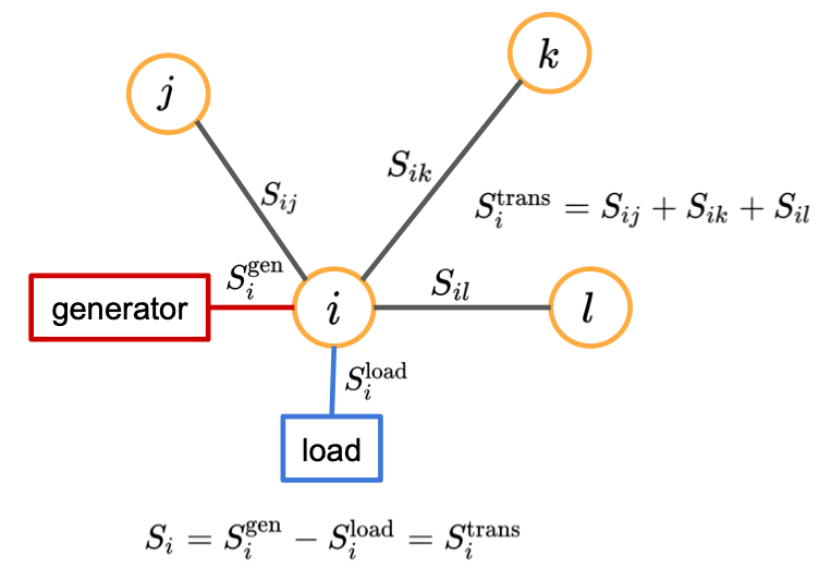Figure 3. Power balance and quantities of a bus connected to three adjacent buses and including a single generator and a single load.

Tellegen’s theorem establishes a simple relationship between these power quantities:

\[\begin{equation} S_{i} = S_{i}^{\mathrm{gen}} - S_{i}^{\mathrm{load}} = S_{i}^{\mathrm{trans}} \ \ \ \ \forall i \in \mathcal{N}. \label{power_balance} \end{equation}\]

Eq. \(\eqref{power_balance}\) expresses the law of conservation of power (energy): the power injected (\(S_{i}^{\mathrm{gen}}\)) to bus \(i\) must be equal to the power going out from the bus, i.e. the sum of the withdrawn (\(S_{i}^{\mathrm{load}}\)) and transmitted power (\(S_{i}^{\mathrm{trans}}\)). In the most basic model, a bus can represent either a generator (i.e. \(S_{i} = S_{i}^{\mathrm{gen}}\)) or a load (i.e. \(S_{i} = -S_{i}^{\mathrm{load}}\)). For a given bus, the transmitted power can be obtained simply as a sum of the powers flowing in to and out from the bus, \(S_{i}^{\mathrm{trans}} = \sum \limits_{j \in \mathcal{N}_{i}} S_{ij}\). Therefore, the basic BIM has the following concise form:

\[\begin{equation} S_{i} = \sum \limits_{j \in \mathcal{N}_{i}} Y_{ij}^{*} \left( |V_{i}|^{2} - V_{i}V_{j}^{*} \right) \ \ \ \ \forall i \in \mathcal{N} . \label{bim_basic_concise} \end{equation}\]

Branch flow model

We briefly describe an alternative formulation of the power flow problem, the branch flow model (BFM).⁵ The BFM is based on the directed graph representation of the grid network, \(\mathbb{G}_{D}\), and directly models branch flows and currents. Let us fix an arbitrary orientation of \(\mathbb{G}_{D}\) and let \((i, j) \in \mathcal{E}\) denote an edge pointing from bus \(i\) to bus \(j\). Then, the BFM is defined by the following set of complex equations:

\[\begin{equation} \left\{ \begin{aligned} S_{i} & = \sum \limits_{(i, j) \in \mathcal{E}_{D}} S_{ij} - \sum \limits_{(k, i) \in \mathcal{E}} \left( S_{ki} - Z_{ki} |I_{ki}|^{2} \right) & \forall i \in \mathcal{N}, \\ I_{ij} & = Y_{ij} \left( V_{i} - V_{j} \right) & \forall (i, j) \in \mathcal{E}, \\ S_{ij} & = V_{i}I_{ij}^{*} & \forall (i, j) \in \mathcal{E}, \\ \end{aligned} \right. \label{bfm_basic_concise} \end{equation}\]

where the first, second and third sets of equations correspond to the power balance, Ohm’s law, and branch power definition, respectively.

The power flow problem

The power flow problem is to find a unique solution of a power system (given certain input variables) and, therefore, it is central to power grid analysis.

First, let us consider the BIM equations (eq. \(\eqref{bim_basic_concise}\)) that define a complex non-linear system with \(N = |\mathcal{N}|\) complex equations, and \(2N\) complex variables, \(\left\{S_{i}, V_{i}\right\}_{i=1}^{N}\). Equivalently, either using the admittance (eq. \(\eqref{power_flow_y}\)) or the impedance (eq. \(\eqref{power_flow_z}\)) components we can construct \(2N\) real equations with \(4N\) real variables: \(\left\{p_{i}, q_{i}, v_{i}, \delta_{i}\right\}_{i=1}^{N}\), where \(S_{i} = p_{i} + \mathrm{j}q_{i}\). The power flow problem is the following: for each bus we specify two of the four real variables and then using the \(2N\) equations we derive the remaining variables. Depending on which variables are specified there are three basic types of buses:

• Slack (or \(V\delta\) bus) is usually a reference bus, where the voltage angle and magnitude are specified. Also, slack buses are used to make up any generation and demand mismatch caused by line losses. The voltage angle is usually set to 0, while the magnitude to 1.0 per unit.
• Load (or \(PQ\) bus) is the most common bus type, where only demand but no power generation takes place. For such buses the active and reactive powers are specified.
• Generator (or \(PV\) bus) specifies the active power and voltage magnitude variables.
  
  

Table 1. Basic bus types in power flow problem.

Bus type	Code	Specified variables
Slack	\(V\delta\)	\(v_{i}\), \(\delta_{i}\)
Load	\(PQ\)	\(p_{i}\), \(q_{i}\)
Generator	\(PV\)	\(p_{i}\), \(v_{i}\)

Further, let \(E = |\mathcal{E}|\) denote the number of directed edges. The BFM formulation (eq. \(\eqref{bfm_basic_concise}\)) includes \(N + 2E\) complex equations with \(2N + 2E\) complex variables: \(\left\{ S_{i}, V_{i} \right\}_{i \in \mathcal{N}} \cup \left\{ S_{ij}, I_{ij} \right\}_{(i, j) \in \mathcal{E}}\) or equivalently, \(2N + 4E\) real equations with \(4N + 4E\) real variables.

BIM vs BFM

The BIM and the BFM are equivalent formulations, i.e. they define the same physical problem and provide the same solution.⁶ Although the formulations are equivalent, in practice we might prefer one model over the other. Depending on the actual problem and the structure of the system, it might be easier to obtain results and derive an exact solution or an approximate relaxation from one formulation than from the other one.

Table 2. Comparison of basic BIM and BFM formulations: complex variables, number of complex variables and equations. Corresponding real variables, their numbers as well as the number of real equations are also shown in parentheses.

Formulation	Variables	Number of variables	Number of equations
BIM	\(V_{i} \ (v_{i}, \delta_{i})\) \(S_{i} \ (p_{i}, q_{i})\)	\(2N\) \((4N)\)	\(N\) \((2N)\)
BFM	\(V_{i} \ (v_{i}, \delta_{i})\) \(S_{i} \ (p_{i}, q_{i})\) \(I_{ij} \ (i_{ij}, \gamma_{ij})\) \(S_{ij} \ (p_{ij}, q_{ij})\)	\(2N + 2E\) \((4N + 4E)\)	\(N + 2E\) \((2N + 4E)\)

Solving the power flow problem

Power flow problems (formulated as either a BIM or a BFM) define a non-linear system of equations. There are multiple approaches to solve power flow systems but the most widely used technique is the Newton–Raphson method. Below we demonstrate how it can be applied to the BIM formulation. First, we rearrange eq. \(\eqref{bim_basic_concise}\):

\[\begin{equation} F_{i} = S_{i} - \sum \limits_{j \in \mathcal{N}_{i}} Y_{ij}^{*} \left( |V_{i}|^{2} - V_{i}V_{j}^{*} \right) = 0 \ \ \ \ \forall i \in \mathcal{N}. \end{equation}\]

The above set of equations can be expressed simply as \(F(X) = 0\), where \(X\) denotes the \(N\) complex or more conveniently, the \(2N\) real unknown variables and \(F\) represents the \(N\) complex or \(2N\) real equations.

In the Newton—Raphson method the solution is sought in an iterative fashion, until a certain threshold of convergence is satisfied. In the \((n+1)\)th iteration we obtain:

\[\begin{equation} X_{n+1} = X_{n} - J_{F}(X_{n})^{-1} F(X_{n}), \end{equation}\]

where \(J_{F}\) is the Jacobian matrix with \(\left[J_{F}\right]_{ij} = \frac{\partial F_{i}}{\partial X_{j}}\) elements. We also note that, instead of computing the inverse of the Jacobian matrix, a numerically more stable approach is to solve first a linear system of \(J_{F}(X_{n}) \Delta X_{n} = -F(X_{n})\) and then obtain \(X_{n+1} = X_{n} + \Delta X_{n}\).

Since Newton—Raphson method requires only the computation of first derivatives of the \(F_{i}\) functions with respect to the variables, this technique is in general very efficient even for large, real-size grids.

Towards more realistic power flow models

In the previous sections we introduced the main concepts needed to understand and solve the power flow problem. However, the derived models were rather basic ones, and real systems require more reasonable approaches. Below we will construct more sophisticated models by extending the basic equations considering the following:

• multiple generators and loads included in buses;
• shunt elements connected to buses;
• modeling transformers and phase shifters;
• modeling asymmetric line charging.

We note that actual power grids can include additional elements besides the ones we discuss.

Improving the bus model

We start with the generated (\(S_{i}^{\mathrm{gen}}\)) and load (\(S_{i}^{\mathrm{load}}\)) powers in the power balance equations, i.e. \(S_{i} = S_{i}^{\mathrm{gen}} - S_{i}^{\mathrm{load}} = S_{i}^{\mathrm{trans}}\) for each bus \(i\). Electric grid buses can actually include multiple generators and loads together. In order to take this structure into account we introduce \(\mathcal{G}_{i}\) and \(\mathcal{L}_{i}\), denoting the set of generators and the set of loads at bus \(i\), respectively. Also, \(\mathcal{G} = \bigcup \limits_{i \in \mathcal{N}} \mathcal{G}_{i}\) and \(\mathcal{L} = \bigcup \limits_{i \in \mathcal{N}} \mathcal{L}_{i}\) indicate the sets of all generators and loads, respectively. Then we can write the following complex-valued expressions:

\[\begin{equation} S_{i}^{\mathrm{gen}} = \sum \limits_{g \in \mathcal{G}_{i}} S_{g}^{G} \ \ \ \ \forall i \in \mathcal{N}, \end{equation}\] \[\begin{equation} S_{i}^{\mathrm{load}} = \sum \limits_{l \in \mathcal{L}_{i}} S_{l}^{L} \ \ \ \ \forall i \in \mathcal{N}, \end{equation}\]

where \(\left\{S_{g}^{G}\right\}_{g \in \mathcal{G}}\) and \(\left\{S_{l}^{L}\right\}_{l \in \mathcal{L}}\) are the complex powers of generator dispatches and load consumptions, respectively. It is easy to see from the equations above that having multiple generators and loads per bus increases the total number of variables, while the number of equations does not change. If the system includes \(N = \lvert \mathcal{N} \rvert\) buses, \(G = \lvert \mathcal{G} \rvert\) generators and \(L = \lvert \mathcal{L} \rvert\) loads, then the total number of complex variables changes to \(N + G + L\) and \(N + G + L + 2E\) for BIM and BFM, respectively.

Buses can also include shunt elements that are used to model connected capacitors and inductors. They are represented by individual admittances resulting in additional power flowing out of the bus:

\[\begin{equation} S_{i} = S_{i}^{\mathrm{gen}} - S_{i}^{\mathrm{load}} - S_{i}^{\mathrm{shunt}} = \sum \limits_{g \in \mathcal{G}_{i}} S_{g}^{G} - \sum \limits_{l \in \mathcal{L}_{i}} S_{l}^{L} - \sum \limits_{s \in \mathcal{S}_{i}} S_{s}^{S} \ \ \ \ \forall i \in \mathcal{N}, \end{equation}\]

where \(\mathcal{S}_{i}\) is the set of shunts attached to bus \(i\) and \(S^{S}_{s} = \left( Y_{s}^{S} \right)^{*} \lvert V_{i} \rvert^{2}\) with admittance \(Y_{s}^{S}\) of shunt \(s \in \mathcal{S}_{i}\). Shunt elements do not introduce additional variables in the system.

Improving the branch model

In real power grids, branches can be transmission lines, transformers, or phase shifters. Transformers are used to control voltages, active and, sometimes, reactive power flows. In this section we take the transformer and line charging also into account by a general branch model (Figure 4).

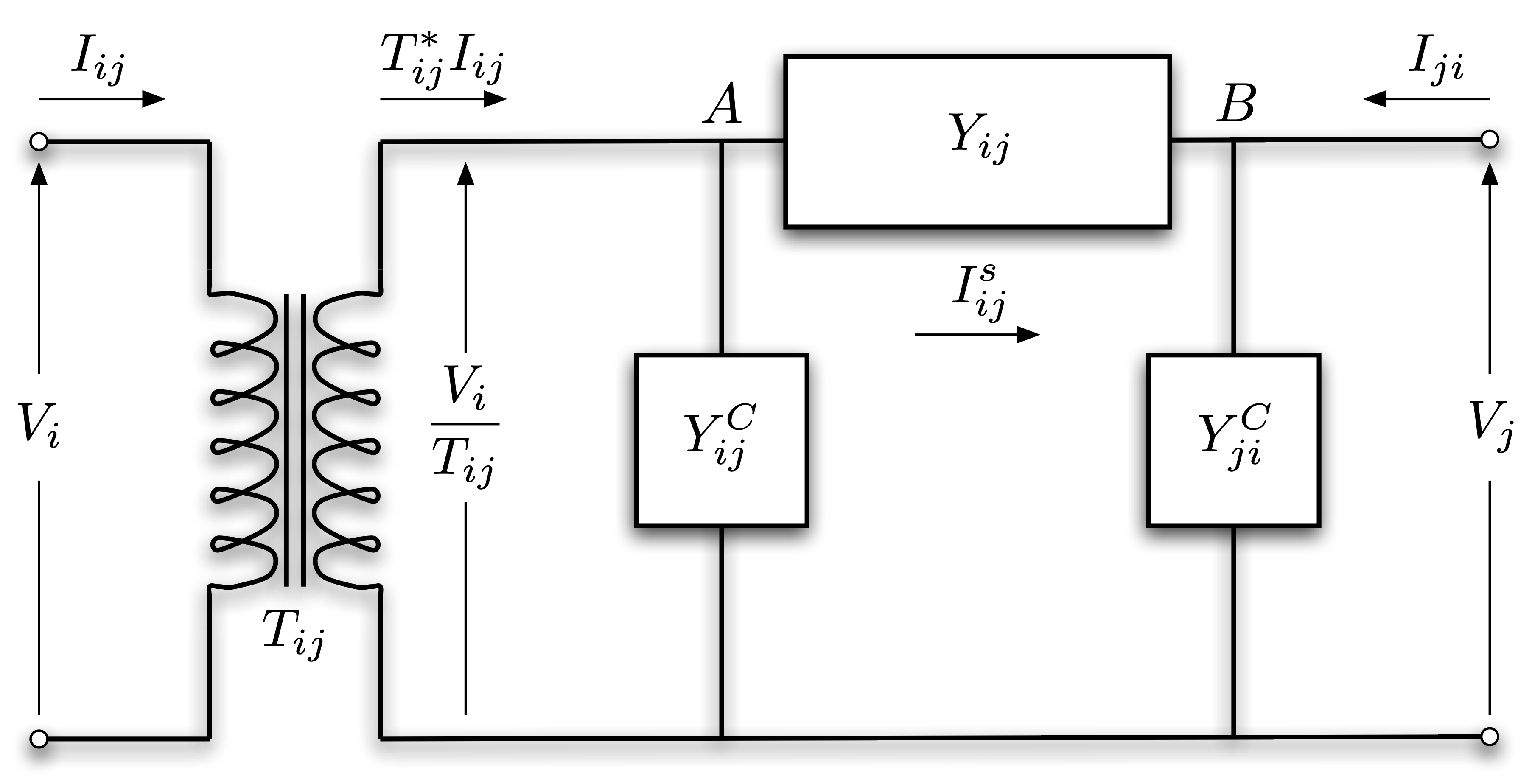Figure 4. General branch model including transformers and \(\pi\)-section model (source: MATPOWER manual⁷).

Transformers (and also phase shifters) are represented by the complex tap ratio \(T_{ij}\), or equivalently, by its magnitude \(t_{ij}\) and phase angle \(\theta_{ij}\). Also, line charging is usually modeled by the \(\pi\) transmission line (or \(\pi\)-section) model, which places shunt admittances at the two ends of the transmission line, beside its series admittance. We will treat the shunt admittances in a fairly general way, i.e. \(Y_{ij}^{C}\) and \(Y_{ji}^{C}\) are not necessarily equal but we also note that a widely adopted practice is to assume equal values and consider their susceptance component only. Since this model is not symmetric anymore, for consistency we introduce the following convention: we select the orientation of each branch \((i, j) \in \mathcal{E}\) that matches the structure presented in Figure 4.

In order to derive the corresponding power flow equations of this model (for both directions due to the asymmetric arrangement), we first look for expressions of the current \(I_{ij}\) and \(I_{ji}\).
The transformer alters the input voltage \(V_{i}\) and current \(I_{ij}\). Using the complex tap ratio the output voltage and current are \(\frac{V_{i}}{T_{ij}}\) and \(T_{ij}^{*}I_{ij}\), respectively. Let \(I_{ij}^{s}\) denote the series current flowing between point \(A\) and \(B\) in Figure 4. Based on Kirchhoff’s current law the net current flowing into node \(A\) is equal to the net current flowing out from it, i.e. \(T_{ij}^{*} I_{ij} = I_{ij}^{s} + Y_{ij}^{C} \frac{V_{i}}{T_{ij}}\). Rearranging this expression for \(I_{ij}\) we get:

\[\begin{equation} I_{ij} = \frac{I_{ij}^{s}}{T_{ij}^{*}} + Y_{ij}^{C} \frac{V_{i}}{\lvert T_{ij} \rvert^{2}} \quad \forall (i, j) \in \mathcal{E}. \end{equation}\]

Similarly, applying Kirchhoff’s current law for node \(B\) we can obtain \(I_{ji}\):

\[\begin{equation} I_{ji} = -I_{ij}^{s} + Y_{ji}^{C} V_{j} \quad \forall (j, i) \in \mathcal{E}^{R}. \end{equation}\]

Finally, using again Ohm’s law, the series current has the following simple expression: \(I_{ij}^{s} = Y_{ij} \left( \frac{V_{i}}{T_{ij}} - V_{j} \right)\). Now we can easily obtain the corresponding power flows:

\[\begin{equation} \begin{aligned} S_{ij} & = V_{i}I_{ij}^{*} = V_{i} \left( \frac{I_{ij}^{s}}{T_{ij}^{*}} + Y_{ij}^{C} \frac{V_{i}}{\lvert T_{ij} \rvert^{2}}\right)^{*} & \\ & = Y_{ij}^{*} \left( \frac{\lvert V_{i} \rvert^{2}}{\lvert T_{ij} \rvert^{2}} - \frac{V_{i} V_{j}^{*}}{T_{ij}} \right) + \left( Y_{ij}^{C} \right)^{*} \frac{\lvert V_{i} \rvert^{2}}{\lvert T_{ij} \rvert^{2}} \ \ \ \ & \forall (i, j) \in \mathcal{E} \\ S_{ji} & = V_{j}I_{ji}^{*} = V_{j} \left( -I_{ij}^{s} + Y_{ji}^{C}V_{j} \right)^{*} & \\ & = Y_{ij}^{*} \left( \lvert V_{j} \rvert^{2} - \frac{V_{j}V_{i}^{*}}{T_{ij}^{*}} \right) + \left( Y_{ji}^{C} \right)^{*} \lvert V_{j} \rvert^{2} \ \ \ \ & \forall (j, i) \in \mathcal{E}^{R} \\ \end{aligned} \end{equation}\]

Improved BIM and BFM models

Putting everything together from the previous sections we present the improved BIM and BFM models:

BIM:

\[\begin{equation} \begin{aligned} \sum \limits_{g \in \mathcal{G}_{i}} S_{g}^{G} - \sum \limits_{l \in \mathcal{L}_{i}} S_{l}^{L} - \sum \limits_{s \in \mathcal{S}_{i}} \left( Y_{s}^{S} \right)^{*} \lvert V_{i} \rvert^{2} = \sum \limits_{(i, j) \in \mathcal{E}} Y_{ij}^{*} \left( \frac{\lvert V_{i} \rvert^{2}}{\lvert T_{ij} \rvert^{2}} - \frac{V_{i} V_{j}^{*}}{T_{ij}} \right) + \left( Y_{ij}^{C} \right)^{*} \frac{\lvert V_{i} \rvert^{2}}{\lvert T_{ij} \rvert^{2}} \\ + \sum \limits_{(k, i) \in \mathcal{E}^{R}} Y_{ik}^{*} \left( \lvert V_{k} \rvert^{2} - \frac{V_{k}V_{i}^{*}}{T_{ik}^{*}} \right) + \left( Y_{ki}^{C} \right)^{*} \lvert V_{k} \rvert^{2} \ \ \ \ \forall i \in \mathcal{N}, \\ \end{aligned} \label{bim_concise} \end{equation}\]

where, on the left-hand side, the net power at bus \(i\) is computed from the power injection of multiple generators and power withdrawals of multiple loads and shunt elements, while, on the right-hand side, the transmitted power is a sum of the outgoing (first term) and incoming (second term) power flows to and from the corresponding adjacent buses.

BFM:

\[\begin{equation} \begin{aligned} & \sum \limits_{g \in \mathcal{G}_{i}} S_{g}^{G} - \sum \limits_{l \in \mathcal{L}_{i}} S_{l}^{L} - \sum \limits_{s \in \mathcal{S}_{i}} \left( Y_{s}^{S} \right)^{*} \lvert V_{i} \rvert^{2} = \sum \limits_{(i, j) \in \mathcal{E}} S_{ij} + \sum \limits_{(k, i) \in \mathcal{E}^{R}} S_{ki} & \forall i \in \mathcal{N} \\ & I_{ij}^{s} = Y_{ij} \left( \frac{V_{i}}{T_{ij}} - V_{j} \right) & \forall (i, j) \in \mathcal{E} \\ & S_{ij} = V_{i} \left( \frac{I_{ij}^{s}}{T_{ij}^{*}} + Y_{ij}^{C} \frac{V_{i}}{\lvert T_{ij} \rvert^{2}}\right)^{*} & \forall (i, j) \in \mathcal{E} \\ & S_{ji} = V_{j} \left( -I_{ij}^{s} + Y_{ji}^{C}V_{j} \right)^{*} & \forall (j, i) \in \mathcal{E}^{R} \\ \end{aligned} \label{bfm_concise} \end{equation}\]

As before, BFM is an equivalent formulation to BIM (first set of equations), with the only difference being that BFM treats the series currents (second set of equations) and power flows (third and fourth sets of equations) as explicit variables.

Table 3. Comparison of improved BIM and BFM formulations: complex variables, number of complex variables and equations. Corresponding real variables, their numbers as well as the number of real equations are also shown in parentheses.

Formulation	Variables	Number of variables	Number of equations
BIM	\(V_{i} \ (v_{i}, \delta_{i})\) \(S_{g}^{G} \ (p_{g}^{G}, q_{g}^{G})\) \(S_{l}^{L} \ (p_{l}^{L}, q_{l}^{L})\)	\(N + G + L\) \((2N + 2G + 2L)\)	\(N\) \((2N)\)
BFM	\(V_{i} \ (v_{i}, \delta_{i})\) \(S_{g}^{G} \ (p_{g}^{G}, q_{g}^{G})\) \(S_{l}^{L} \ (p_{l}^{L}, q_{l}^{L})\) \(I_{ij}^{s} \ (i_{ij}^{s}, \gamma_{ij}^{s})\) \(S_{ij} \ (p_{ij}, q_{ij})\) \(S_{ji} \ (p_{ji}, q_{ji})\)	\(N + G + L + 3E\) \((2N + 2G + 2L + 6E)\)	\(N + 3E\) \((2N + 6E)\)

Conclusions

In this blog post, we introduced the main concepts of the power flow problem and derived the power flow equations for a basic and a more realistic model using two equivalent formulations. We also showed that the resulting mathematical problems are non-linear systems that can be solved by the Newton—Raphson method.

Solving power flow problems is essential for the analysis of power grids. Based on a set of specified variables, the power flow solution provides the unknown ones. Consider a power grid with \(N\) buses, \(G\) generators and \(L\) loads, and let us specify only the active and reactive powers of the loads, which means \(2L\) number of known real-valued variables. Whichever formulation we use, this system is underdetermined and we would need to specify \(2G\) additional variables (Table 3.) to obtain a unique solution. However, generators have distinct power supply capacities and cost curves, and we can ask an interesting question: among the many physically possible specifications of the generator variables which is the one that would minimize the total economic cost?

This question leads to the mathematical model of economic dispatch, which is one of the most widely used optimal power flow problems. Optimal power flow problems are constrained optimization problems that are based on the power flow equations with additional physical constraints and an objective function. In our next post, we will discuss the main types and components of optimal power flow, and show how exact and approximate solutions can be obtained for these significantly more challenging problems.

---