Linear Models from a Gaussian Process Point of View with Stheno and JAX

Author: Wessel Bruinsma and James Requeima

Cross-posted at wesselb.github.io.

A linear model prescribes a linear relationship between inputs and outputs. Linear models are amongst the simplest of models, but they are ubiquitous across science. A linear model with Gaussian distributions on the coefficients forms one of the simplest instances of a Gaussian process. In this post, we will give a brief introduction to linear models from a Gaussian process point of view. We will see how a linear model can be implemented with Gaussian process probabilistic programming using Stheno, and how this model can be used to denoise noisy observations. (Disclosure: Will Tebbutt and Wessel are the authors of Stheno; Will maintains a Julia version.) In short, probabilistic programming is a programming paradigm that brings powerful probabilistic models to the comfort of your programming language, which often comes with tools to automatically perform inference (make predictions). We will also use JAX’s just-in-time compiler to make our implementation extremely efficient.

Linear Models from a Gaussian Process Point of View

Consider a data set \((x_i, y_i)_{i=1}^n \subseteq \R \times \R\) consisting of \(n\) real-valued input–output pairs. Suppose that we wish to estimate a linear relationship between the inputs and outputs:

where \(a\) is an unknown slope, \(b\) is an unknown offset, and \(\e_i\) is some error/noise associated with the observation \(y_i\). To implement this model with Gaussian process probabilistic programming, we need to cast the problem into a functional form. This means that we will assume that there is some underlying, random function \(y \colon \R \to \R\) such that the observations are evaluations of this function: \(y_i = y(x_i)\). The model for the random function \(y\) will embody the structure of the linear model \eqref{eq:ax_b}. This may sound hard, but it is not difficult at all. We let the random function \(y\) be of the following form:

where \(a\colon \R \to \R\) is a random constant function. An example of a constant function \(f\) is \(f(x) = 5\). Random means that the value \(5\) is not fixed, but modelled with a random value drawn from some probability distribution, because we don’t know the true value. We let \(b\colon \R \to \R\) also be a random constant function, and \(\e\colon \R \to \R\) a random noise function. Do you see the similarities between \eqref{eq:ax_b} and \eqref{eq:ax_b_functional}? If all that doesn’t fully make sense, don’t worry; things should become more clear as we implement the model.

To model random constant functions and random noise functions, we will use Stheno, which is a Python library for Gaussian process modelling. We also have a Julia version, but in this post we’ll use the Python version. To install Stheno, run the command

pip install --upgrade --upgrade-strategy eager stheno

In Stheno, a Gaussian process can be created with GP(kernel), where kernel is the so-called kernel or covariance function of the Gaussian process. The kernel determines the properties of the function that the Gaussian process models. For example, the kernel EQ() models smooth functions, and the kernel Matern12() models functions that look jagged. See the kernel cookbook for an overview of commonly used kernels and the documentation of Stheno for the corresponding classes. For constant functions, you can set the kernel to simply a constant, for example 1, which then models the constant function with a value drawn from \(\mathcal{N}(0, 1)\). (By default, in Stheno, all means are zero; but, if you like, you can also set a mean.)

Let’s start out by creating a Gaussian process for the random constant function \(a(x)\) that models the slope.

>>> from stheno import GP

>>> a = GP(1)

>>> a
GP(0, 1)

You can see how the Gaussian process looks by simply sampling from it. To sample from the Gaussian process a at some inputs x, evaluate it at those inputs, a(x), and call the method sample: a(x).sample(). This shows that you can really think of a Gaussian process just like you think of a function: pass it some inputs to get (the model for) the corresponding outputs.

>>> x = np.linspace(0, 10, 100)

>>> plt.plot(x, a(x).sample(20)); plt.show()

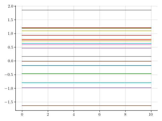Figure 1: Samples of a Gaussian process that models a constant function.

We’ve sampled a bunch of constant functions. Sweet! The next step in the model \eqref{eq:ax_b_functional} is to multiply the slope function \(a(x)\) by \(x\). To multiply a by \(x\), we multiply a by the function lambda x: x, which casts also \(x\) as a function:

>>> f = a * (lambda x: x)

>>> f
GP(0, <lambda>)

This will give rise to functions like \(x \mapsto 0.1x\) and \(x \mapsto -0.4x\), depending on the value that \(a(x)\) takes.

>>> plt.plot(x, f(x).sample(20)); plt.show()

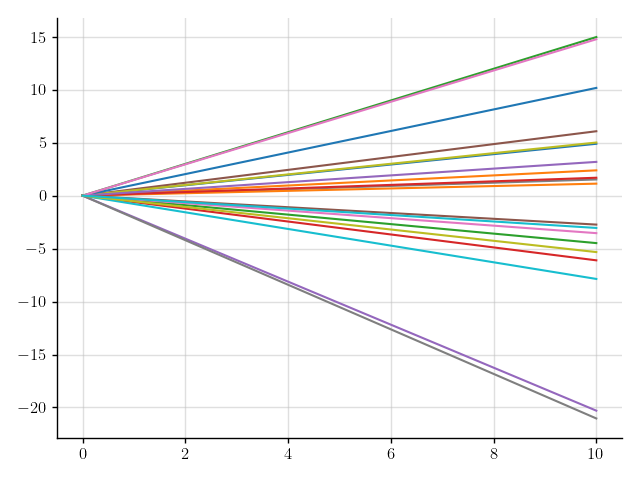Figure 2: Samples of a Gaussian process that models functions with a random slope.

This is starting to look good! The only ingredient that is missing is an offset. We model the offset just like the slope, but here we set the kernel to 10 instead of 1, which models the offset with a value drawn from \(\mathcal{N}(0, 10)\).

>>> b = GP(10)

>>> f = a * (lambda x: x) + b
AssertionError: Processes GP(0, <lambda>) and GP(0, 10 * 1) are associated to different measures.

Something went wrong. Stheno has an abstraction called measures, where only GPs that are part of the same measure can be combined into new GPs; the abstraction of measures is there to keep things safe and tidy. What goes wrong here is that a and b are not part of the same measure. Let’s explicitly create a new measure and attach a and b to it.

>>> from stheno import Measure

>>> prior = Measure()

>>> a = GP(1, measure=prior)

>>> b = GP(10, measure=prior)

>>> f = a * (lambda x: x) + b

>>> f
GP(0, <lambda> + 10 * 1)

Let’s see how samples from f look like.

>>> plt.plot(x, f(x).sample(20)); plt.show()

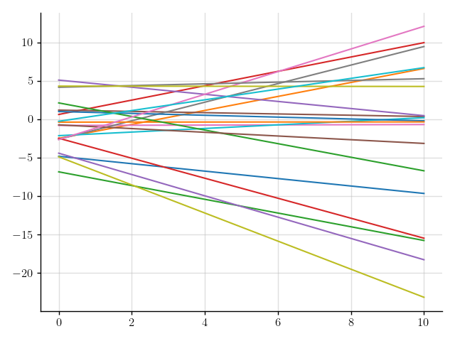Figure 3: Samples of a Gaussian process that models linear functions.

Perfect! We will use f as our linear model.

In practice, observations are corrupted with noise. We can add some noise to the lines in Figure 3 by adding a Gaussian process that models noise. You can construct such a Gaussian process by using the kernel Delta(), which models the noise with independent \(\mathcal{N}(0, 1)\) variables.

>>> from stheno import Delta

>>> noise = GP(Delta(), measure=prior)

>>> y = f + noise

>>> y
GP(0, <lambda> + 10 * 1 + Delta())

>>> plt.plot(x, y(x).sample(20)); plt.show()

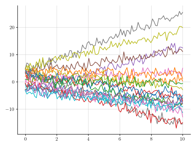Figure 4: Samples of a Gaussian process that models noisy linear functions.

That looks more realistic, but perhaps that’s a bit too much noise. We can tune down the amount of noise, for example, by scaling noise by 0.5.

>>> y = f + 0.5 * noise

>>> y
GP(0, <lambda> + 10 * 1 + 0.25 * Delta())

>>> plt.plot(x, y(x).sample(20)); plt.show()

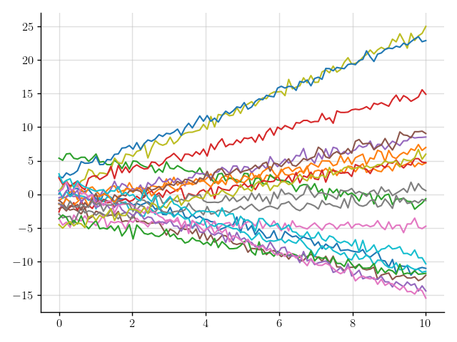Figure 5: Samples of a Gaussian process that models noisy linear functions.

Much better.

To summarise, our linear model is given by

prior = Measure()

a = GP(1, measure=prior)            # Model for slope
b = GP(10, measure=prior)           # Model for offset
f = a * (lambda x: x) + b           # Noiseless linear model

noise = GP(Delta(), measure=prior)  # Model for noise
y = f + 0.5 * noise                 # Noisy linear model

We call a program like this a Gaussian process probabilistic program (GPPP). Let’s generate some noisy synthetic data, (x_obs, y_obs), that will make up an example data set \((x_i, y_i)_{i=1}^n\). We also save the observations without noise added—f_obs—so we can later check how good our predictions really are.

>>> x_obs = np.linspace(0, 10, 50_000)

>>> f_obs = 0.8 * x_obs - 2.5

>>> y_obs = f_obs + 0.5 * np.random.randn(50_000)

>>> plt.scatter(x_obs, y_obs); plt.show()

Figure 6: Some observations.

We will see next how we can fit our model to this data.

Inference in Linear Models

Suppose that we wish to remove the noise from the observations in Figure 6. We carefully phrase this problem in terms of our GPPP: the observations y_obs are realisations of the noisy linear model y at x_obs—realisations of y(x_obs)—and we wish to make predictions for the noiseless linear model f at x_obs—predictions for f(x_obs).

In Stheno, we can make predictions based on observations by conditioning the measure of the model on the observations. In our GPPP, the measure is given by prior, so we aim to condition prior on the observations y_obs for y(x_obs). Mathematically, this process of incorporating information by conditioning happens through Bayes’ rule. Programmatically, we first make an Observations object, which represents the information—the observations—that we want to incorporate, and then condition prior on this object:

>>> from stheno import Observations

>>> obs = Observations(y(x_obs), y_obs)

>>> post = prior.condition(obs)

You can also more concisely perform these two steps at once, as follows:

>>> post = prior | (y(x_obs), y_obs)

This mimics the mathematical notation used for conditioning.

With our updated measure post, which is often called the posterior measure, we can make a prediction for f(x_obs) by passing f(x_obs) to post:

>>> pred = post(f(x_obs))

>>> pred.mean
<dense matrix: shape=50000x1, dtype=float64
 mat=[[-2.498]
      [-2.498]
      [-2.498]
      ...
      [ 5.501]
      [ 5.502]
      [ 5.502]]>

>>> pred.var
<low-rank matrix: shape=50000x50000, dtype=float64, rank=2
 left=[[1.e+00 0.e+00]
       [1.e+00 2.e-04]
       [1.e+00 4.e-04]
       ...
       [1.e+00 1.e+01]
       [1.e+00 1.e+01]
       [1.e+00 1.e+01]]
 middle=[[ 2.001e-05 -2.995e-06]
         [-2.997e-06  6.011e-07]]
 right=[[1.e+00 0.e+00]
        [1.e+00 2.e-04]
        [1.e+00 4.e-04]
        ...
        [1.e+00 1.e+01]
        [1.e+00 1.e+01]
        [1.e+00 1.e+01]]>

The prediction pred is a multivariate Gaussian distribution with a particular mean and variance, which are displayed above. You should view post as a function that assigns a probability distribution—the prediction—to every part of our GPPP, like f(x_obs). Note that the variance of the prediction is a massive matrix of size 50k \(\times\) 50k. Under the hood, Stheno uses structured representations for matrices to compute and store matrices in an efficient way.

Let’s see how the prediction pred for f(x_obs) looks like. The prediction pred exposes the method marginals that conveniently computes the mean and associated lower and upper error bounds for you.

>>> mean, error_bound_lower, error_bound_upper  = pred.marginals()

>>> mean
array([-2.49818708, -2.49802708, -2.49786708, ...,  5.50148996,
        5.50164996,  5.50180997])

>>> error_bound_upper - error_bound_lower
array([0.01753381, 0.01753329, 0.01753276, ..., 0.01761883, 0.01761935,
       0.01761988])

The error is very small—on the order of \(10^{-2}\)—which means that Stheno predicted f(x_obs) with high confidence.

>>> plt.scatter(x_obs, y_obs); plt.plot(x_obs, mean); plt.show()

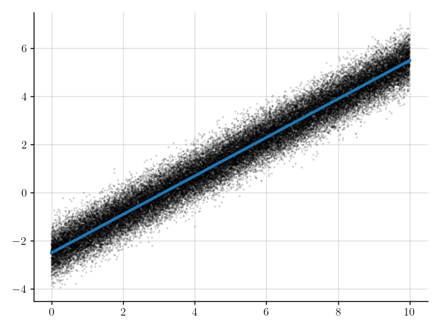Figure 7: Mean of the prediction (blue line) for the denoised observations.

The blue line in Figure 7 shows the mean of the predictions. This line appears to nicely pass through the observations with the noise removed. But let’s see how good the predictions really are by comparing to f_obs, which we previously saved.

>>> f_obs - mean
array([-0.00181292, -0.00181292, -0.00181292, ..., -0.00180997,
       -0.00180997, -0.00180997])

>>> np.mean((f_obs - mean) ** 2)  # Compute the mean square error.
3.281323087544209e-06

That’s pretty close! Not bad at all.

We wrap up this section by encapsulating everything that we’ve done so far in a function linear_model_denoise, which denoises noisy observations from a linear model:

def linear_model_denoise(x_obs, y_obs):
    prior = Measure()
    a = GP(1, measure=prior)            # Model for slope
    b = GP(10, measure=prior)           # Model for offset
    f = a * (lambda x: x) + b           # Noiseless linear model
    noise = GP(Delta(), measure=prior)  # Model for noise
    y = f + 0.5 * noise                 # Noisy linear model

    post = prior | (y(x_obs), y_obs)    # Condition on observations.
    pred = post(f(x_obs))               # Make predictions.
    return pred.marginals()             # Return the mean and associated error bounds.

>>> linear_model_denoise(x_obs, y_obs)
(array([-2.49818708, -2.49802708, -2.49786708, ...,  5.50148996,
        5.50164996,  5.50180997]), array([-2.50695399, -2.50679372, -2.50663346, ...,  5.49268055,
        5.49284029,  5.49300003]), array([-2.48942018, -2.48926044, -2.4891007 , ...,  5.51029937,
        5.51045964,  5.51061991]))

>>> %timeit linear_model_denoise(x_obs, y_obs)
233 ms ± 12.6 ms per loop (mean ± std. dev. of 7 runs, 1 loop each)

To denoise 50k observations, linear_model_denoise takes about 250 ms. Not terrible, but we can do much better, which is important if we want to scale to larger numbers of observations. In the next section, we will make this function really fast.

Making Inference Fast

To make linear_model_denoise fast, firstly, the linear algebra that happens under the hood when linear_model_denoise is called should be simplified as much as possible. Fortunately, this happens automatically, due to the structured representation of matrices that Stheno uses. For example, when making predictions with Gaussian processes, the main computational bottleneck is usually the construction and inversion of y(x_obs).var, the variance associated with the observations:

>>> y(x_obs).var
<Woodbury matrix: shape=50000x50000, dtype=float64
 diag=<diagonal matrix: shape=50000x50000, dtype=float64
       diag=[0.25 0.25 0.25 ... 0.25 0.25 0.25]>
 lr=<low-rank matrix: shape=50000x50000, dtype=float64, rank=2
     left=[[1.e+00 0.e+00]
           [1.e+00 2.e-04]
           [1.e+00 4.e-04]
           ...
           [1.e+00 1.e+01]
           [1.e+00 1.e+01]
           [1.e+00 1.e+01]]
     middle=[[10.  0.]
             [ 0.  1.]]
     right=[[1.e+00 0.e+00]
            [1.e+00 2.e-04]
            [1.e+00 4.e-04]
            ...
            [1.e+00 1.e+01]
            [1.e+00 1.e+01]
            [1.e+00 1.e+01]]>>

Indeed observe that this matrix has particular structure: it is a sum of a diagonal and a low-rank matrix. In Stheno, the sum of a diagonal and a low-rank matrix is called a Woodbury matrix, because the Sherman–Morrison–Woodbury formula can be used to efficiently invert it. Let’s see how long it takes to construct y(x_obs).var and then invert it. We invert y(x_obs).var using LAB, which is automatically installed alongside Stheno and exposes the API to efficiently work with structured matrices.

>>> import lab as B

>>> %timeit B.inv(y(x_obs).var)
28.5 ms ± 1.69 ms per loop (mean ± std. dev. of 7 runs, 10 loops each)

That’s only 30 ms! Not bad, for such a big matrix. Without exploiting structure, a 50k \(\times\) 50k matrix takes 20 GB of memory to store and about an hour to invert.

Secondly, we would like the code implemented by linear_model_denoise to be as efficient as possible. To achieve this, we will use JAX to compile linear_model_denoise with XLA, which generates blazingly fast code. We start out by importing JAX and loading the JAX extension of Stheno.

>>> import jax

>>> import jax.numpy as jnp

>>> import stheno.jax  # JAX extension for Stheno

We use JAX’s just-in-time (JIT) compiler jax.jit to compile linear_model_denoise:

>>> linear_model_denoise_jitted = jax.jit(linear_model_denoise)

Let’s see what happens when we run linear_model_denoise_jitted. We must pass x_obs and y_obs as JAX arrays to use the compiled version.

>>> linear_model_denoise_jitted(jnp.array(x_obs), jnp.array(y_obs))
Invalid argument: Cannot bitcast types with different bit-widths: F64 => S32.

Oh no! What went wrong is that the JIT compiler wasn’t able to deal with the complicated control flow from the automatic linear algebra simplifications. Fortunately, there is a simple way around this: we can run the function once with NumPy to see how the control flow should go, cache that control flow, and then use this cache to run linear_model_denoise with JAX. Sounds complicated, but it’s really just a bit of boilerplate:

>>> import lab as B

>>> control_flow_cache = B.ControlFlowCache()

>>> control_flow_cache
<ControlFlowCache: populated=False>

Here populated=False means that the cache is not yet populated. Let’s populate it by running linear_model_denoise once with NumPy:

>>> with control_flow_cache:
        linear_model_denoise(x_obs, y_obs)

>>> control_flow_cache
<ControlFlowCache: populated=True>

We now construct a compiled version of linear_model_denoise that uses the control flow cache:

@jax.jit
def linear_model_denoise_jitted(x_obs, y_obs):
    with control_flow_cache:
        return linear_model_denoise(x_obs, y_obs)

>>> linear_model_denoise_jitted(jnp.array(x_obs), jnp.array(y_obs))
(DeviceArray([-2.4981871 , -2.4980271 , -2.49786709, ...,  5.50149004,
              5.50165005,  5.50181005], dtype=float64), DeviceArray([-2.5069514 , -2.50679114, -2.50663087, ...,  5.4927699 ,
              5.49292964,  5.49308938], dtype=float64), DeviceArray([-2.4894228 , -2.48926306, -2.48910332, ...,  5.51021019,
              5.51037046,  5.51053072], dtype=float64))

Nice! Let’s see how much faster linear_model_denoise_jitted is:

>>> %timeit linear_model_denoise(x_obs, y_obs)
233 ms ± 12.6 ms per loop (mean ± std. dev. of 7 runs, 1 loop each)

>>> %timeit linear_model_denoise_jitted(jnp.array(x_obs), jnp.array(y_obs))
1.63 ms ± 16.5 µs per loop (mean ± std. dev. of 7 runs, 1000 loops each)

The compiled function linear_model_denoise_jitted only takes 2 ms to denoise 50k observations! Compared to linear_model_denoise, that’s a speed-up of two orders of magnitude.

Conclusion

We’ve seen how a linear model can be implemented with a Gaussian process probabilistic program (GPPP) using Stheno. Stheno allows us to focus on model construction, and takes away the distraction of the technicalities that come with making predictions. This flexibility, however, comes at the cost of some complicated machinery that happens in the background, such as structured representations of matrices. Fortunately, we’ve seen that this overhead can be completely avoided by compiling your program using JAX, which can result in extremely efficient implementations. To close this post and to warm you up for what’s further possible with Gaussian process probabilistic programming using Stheno, the linear model that we’ve built can easily be extended to, for example, include a quadratic term:

def quadratic_model_denoise(x_obs, y_obs):
    prior = Measure()
    a = GP(1, measure=prior)            # Model for slope
    b = GP(1, measure=prior)            # Model for coefficient of quadratic term
    c = GP(10, measure=prior)           # Model for offset
    # Noiseless quadratic model
    f = a * (lambda x: x) + b * (lambda x: x ** 2) + c
    noise = GP(Delta(), measure=prior)  # Model for noise
    y = f + 0.5 * noise                 # Noisy quadratic model

    post = prior | (y(x_obs), y_obs)    # Condition on observations.
    pred = post(f(x_obs))               # Make predictions.
    return pred.marginals()             # Return the mean and associated error bounds.

To use Gaussian process probabilistic programming for your specific problem, the main challenge is to figure out which model you need to use. Do you need a quadratic term? Maybe you need an exponential term! But, using Stheno, implementing the model and making predictions should then be simple.