Gaussian Processes: from one to many outputs

19 Feb 2021

Author: Eric Perim, Wessel Bruinsma, and Will Tebbutt

This is the first post in a three-part series we are preparing on multi-output Gaussian Processes. Gaussian Processes (GPs) are a popular tool in machine learning, and a technique that we routinely use in our work. Essentially, GPs are a powerful Bayesian tool for regression problems (which can be extended to classification problems through some modifications). As a Bayesian approach, GPs provide a natural and automatic mechanism to construct and calibrate uncertainties. Naturally, getting well-calibrated uncertainties is not easy and depends on a combination of how well the model matches the data and on how much data is available. Predictions made using GPs are not just point predictions: they are whole probability distributions, which is convenient for downstream tasks. There are several good references for those interested in learning more about the benefits of Bayesian methods, from introductory blog posts to classical books.

In this post (and in the forthcoming ones in this series), we are going to assume that the reader has some level of familiarity with GPs in the single-output setting. We will try to keep the maths to a minimum, but will rely on mathematical notation whenever that helps making the message clear. For those who are interested in an introduction to GPs—or just a refresher—we point towards other resources. For a rigorous and in-depth introduction, the book by Rasmussen and Williams stands as one of the best references (and it is made freely available in electronic form by the authors).

We will start by discussing the extension of GPs from one to multiple dimensions, and review popular (and powerful) approaches from the literature. In the following posts, we will look further into some powerful tricks that bring improved scalability and will also share some of our code.

Multi-output GPs

While most people with a background in machine learning or statistics are familiar with GPs, it is not uncommon to have only encountered their single-output formulation. However, many interesting problems require the modelling of multiple outputs instead of just one. Fortunately, it is simple to extend single-output GPs to multiple outputs, and there are a few different ways of doing so. We will call these constructions multi-output GPs (MOGPs).

An example application of a MOGP might be to predict both temperature and humidity as a function of time. Sometimes we might want to include binary or categorical outputs as well, but in this article we will limit the discussion to real-valued outputs. (MOGPs are also sometimes called multi-task GPs, in which case an output is instead referred to as a task. But the idea is the same.) Moreover we will refer to inputs as time, as in the time series setting, but all the discussion in here is valid for any kind of input.

The simplest way to extend GPs to multi-output problems is to model each of the outputs independently, with single-output GPs. We call this model IGPs (for independent GPs). While conceptually simple, computationally cheap, and easy to implement, this approach fails to account for correlations between outputs. If the outputs are correlated, knowing one can provide useful information about others (as we illustrate below), so assuming independence can hurt performance and, in many cases, limit it to being used as a baseline.

To define a general MOGP, all we have to do is to also specify how the outputs covary. Perhaps the simplest way of doing this is by prescribing an additional covariance function (kernel) over outputs, \(k_{\mathrm{o}}(i, j)\), which specifies the covariance between outputs \(i\) and \(j\). Combining this kernel over outputs with a kernel over inputs, e.g. \(k_{\mathrm{t}}(t, t')\), the full kernel of the MOGP is then given by

\[\begin{equation} k((i, t), (j, t')) = \operatorname{cov}(f_i(t), f_j(t')) = k_{\mathrm{o}}(i, j) k_{\mathrm{t}}(t, t'), \end{equation}\]

which says that the covariance between output \(i\) at input \(t\) and output \(j\) at input \(t'\) is equal to the product \(k_{\mathrm{o}}(i, j) k_{\mathrm{t}}(t, t')\). When the kernel \(k((i, t), (j, t'))\) is a product between a kernel over outputs \(k_{\mathrm{o}}(i, j)\) and a kernel over inputs \(k_{\mathrm{t}}(t,t’)\), the kernel \(k((i, t), (j, t'))\) is called separable. In the general case, the kernel \(k((i, t), (j, t'))\) does not have to be separable, i.e. it can be any arbitrary positive-definite function.

Contrary to IGPs, general MOGPs do model correlations between outputs, which means that they are able to use observations from one output to better predict another output. We illustrate this below by contrasting the predictions for two of the outputs in the EEG dataset, one observed and one not observed, using IGPs and another flavour of MOGPs, the ILMM, which we will discuss in detail in the next section. Contrary to the independent GP (IGP), the ILMM is able to successfully predict F2 by exploiting the observations for F3 (and other outputs not shown).

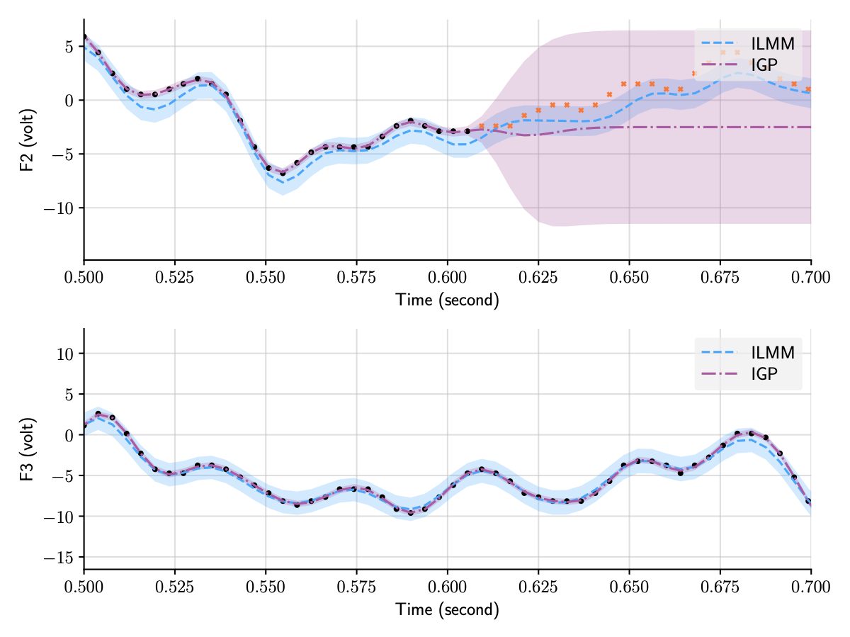Figure 1: Predictions for two of the outputs in the EEG dataset using two distinct MOGP approaches, the ILMM and the IGP. All outputs are modelled jointly, but we only plot two of them for clarity.

Equivalence to single-output GPs

An interesting thing to notice is that a general MOGP kernel is just another kernel, like those used in single-output GPs, but one that now operates on an extended input space (because it also takes in \(i\) and \(j\) as input). Mathematically, say one wants to model \(p\) outputs over some input space \(\mathcal{T}\). By also letting the index of the output be part of the input, we can construct this extended input space: \(\mathcal{T}_{\mathrm{ext}} = \{1,...,p\} \times \mathcal{T}\). Then, a multi-output Gaussian process (MOGP) can be defined via a mean function, \(m\colon \mathcal{T}_{\mathrm{ext}} \to \mathbb{R}\), and a kernel, \(k\colon \mathcal{T}_{\mathrm{ext}}^2 \to \mathbb{R}\). Under this construction it is clear that any property of single-output GPs immediately transfers to MOGPs, because MOGPs can simply be seen as single-output GPs on an extended input space.

An equivalent formulation of MOGPs can be obtained by stacking the multiple outputs into a vector, creating a vector-valued GP. It is sometimes helpful to view MOGPs from this perspective, in which the multiple outputs are viewed as one multidimensional output. We can use this equivalent formulation to define MOGP via a vector-valued mean function, \(m\colon \mathcal{T} \to \mathbb{R}^p\), and a matrix-valued kernel, \(k\colon\mathcal{T}^2 \to \mathbb{R}^{p \times p}\). This mean function and kernel are not defined on the extended input space; rather, in this equivalent formulation, they produce multi-valued outputs. The vector-valued mean function corresponds to the mean of the vector-valued GP, \(m(t) = \mathbb{E}[f(t)]\), and the matrix-valued kernel to the covariance matrix of vector-valued GP, \(k(t, t’) = \mathbb{E}[(f(t) - m(t))(f(t’) - m(t’))^\top]\). When the matrix-valued kernel is evaluated at \(t = t’\), the resulting matrix \(k(t, t) = \mathbb{E}[(f(t) - m(t))(f(t) - m(t))^\top]\) is sometimes called the instantaneous spatial covariance: it describes a covariance between different outputs at a given point in time \(t\).

Because MOGPs can be viewed as single-output GPs on an extended input space, inference works exactly the same way. However, by extending the input space we exacerbate the scaling issues inherent with GPs, because the total number of observations is counted by adding the numbers of observations for each output, and GPs scale badly in the number of observations. While inference in the single-output setting requires the inversion of an \(n \times n\) matrix (where \(n\) is the number of data points), in the case of \(p\) outputs, assuming that at all times all outputs are observed,¹ this turns into the inversion of an \(np \times np\) matrix (assuming the same number of input points for each output as in the single output case), which can quickly become computationally intractable (i.e. not feasible to compute with limited computing power and time). That is because the inversion of a \(q \times q\) matrix takes \(\mathcal{O}(q^3)\) time and \(\mathcal{O}(q^2)\) memory, meaning that time and memory performance will scale, respectively, cubically and quadratically on the number of points in time, \(n\), and outputs, \(p\). In practice this scaling characteristic limits the application of this general MOGP formulation to data sets with very few outputs and data points.

Low-rank approximations

A popular and powerful approach to making MOGPs computationally tractable is to impose a low-rank structure over the covariance between outputs. That is equivalent to assuming that the data can be described by a set of latent (unobserved) Gaussian processes in which the number of these latent processes is fewer than the number of outputs. This builds a simpler lower-dimensional representation of the data. The structure imposed over the covariance matrices through this lower-dimensional representation of the data can be exploited to perform the inversion operation more efficiently (we are going to discuss in detail one of these cases in the next post of this series). There are a variety of different ways in which this kind of structure can be imposed, leading to an interesting class of models which we discuss in the next section.

This kind of assumption is typically used to make the method computationally cheaper. However, these assumptions do bring extra inductive bias to the model. Introducing inductive bias can be a powerful tool in making the model more data-efficient and better-performing in practice, provided that such assumptions are adequate to the particular problem at hand. For instance, low-rank data occurs naturally in different settings. This also happens to be true in electricity grids, due to the mathematical structure of the price-forming process. To make good choices about the kind of inductive bias to use, experience, domain knowledge, and familiarity with the data can be helpful.

The Mixing Model Hierarchy

Models that use a lower-dimensional representation for data have been present in the literature for a long time. Well-known examples include factor analysis, PCA, and VAEs. Even if we restrict ourselves to GP-based models there are still a significant number of notable and powerful models that make this simplifying assumption in one way or another. However, models in the class of MOGPs that explain the data with a lower-dimensional representation are often framed in many distinct ways, which may obscure their relationship and overarching structure. Thus, it is useful to try to look at all these models under the same light, forming a well-defined family that highlights their similarities and differences.

In one of the appendices of a recent paper of ours,² we presented what we called the Mixing Model Hierarchy (MMH), an attempt at a unifying presentation of this large class of MOGP models. It is important to stress that our goal with the Mixing Model Hierarchy is only to organise a large number of pre-existing models from the literature in a reasonably general way, and not to present new models nor claim ownership over important contributions made by other researchers. Further down in this article we present a diagram that connects several relevant papers to the models from the MMH.

The simplest model from the Mixing Model Hierarchy is what we call the Instantaneous Linear Mixing Model (ILMM), which, despite its simplicity, is still a rather general way of describing low-rank covariance structures. In this model the observations are described as a linear combination of the latent processes (i.e. unobserved stochastic processes), given by a set of constant weights. That is, we can write \(f(t) | x, H = Hx(t)\),³ where \(f\) are the observations, \(H\) is a matrix of weights, which we call the mixing matrix, and \(x(t)\) represents the (time-dependent) latent processes—note that we use \(x\) here to denote an unobserved (latent) stochastic process, not an input, which is represented by \(t\). If the latent processes \(x(t)\) are described as GPs, then due to the fact that linear combinations of Gaussian variables are also Gaussian, \(f(t)\) will also be a (MO)GP.

The top-left part of the figure below illustrates the graphical model for the ILMM.⁴ The graphical model highlights the two restrictions imposed by the ILMM when compared with a general MOGP: (i) the instantaneous spatial covariance of \(f\), \(\mathbb{E}[f(t) f^\top(t)] = H H^\top\), does not vary with time, because neither \(H\) nor \(K(t, t) = I_m\) varies with time; and (ii) the noise-free observation \(f(t)\) is a function of \(x(t')\) for \(t'=t\) only, meaning that, for example, \(f\) cannot be \(x\) with a delay or a smoothed version of \(x\). Reflecting this, we call the ILMM a time-invariant (due to (i)) and instantaneous (due to (ii)) MOGP.

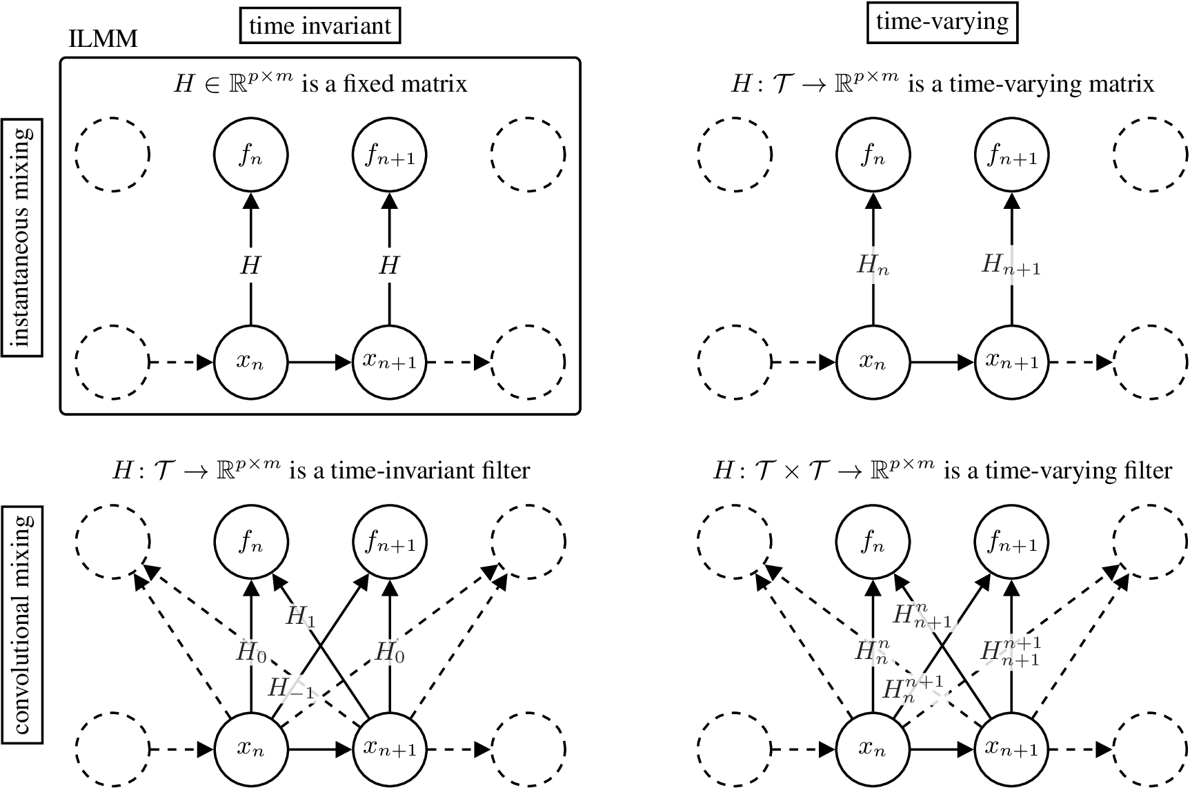Figure 2: Graphical model for different models in the MMH.⁴

There are three general ways in which we can generalise the ILMM within the MMH. The first one is to allow the mixing matrix \(H\) to vary in time. That means that the amount each latent process contributes to each output varies in time. Mathematically, \(H \in \R^{p \times m}\) becomes a matrix-valued function \(H\colon \mathcal{T} \to \R^{p \times m}\), and the mixing mechanism becomes

\[\begin{equation} f(t)\cond H, x = H(t) x(t). \end{equation}\]

We call such MOGP models time-varying. Their graphical model is shown in the figure above, on the top right corner.

A second way to generalise the ILMM is to assume that \(f(t)\) depends on \(x(t')\) for all \(t' \in \mathcal{T}\). That is to say that, at a given time, each output may depend on the values of the latent processes at any other time. We say that these models become non-instantaneous. The mixing matrix \(H \in \R^{p \times m}\) becomes a matrix-valued time-invariant filter \(H\colon \mathcal{T} \to \R^{p \times m}\), and the mixing mechanism becomes

\[\begin{equation} f(t)\cond H, x = \int H(t - \tau) x(\tau) \mathrm{d\tau}. \end{equation}\]

We call such MOGP models convolutional. Their graphical model is shown in the figure above, in the bottom left corner.

A third generalising assumption that we can make is that \(f(t)\) depends on \(x(t')\) for all \(t' \in \mathcal{T}\) and this relationship may vary with time. This is similar to the previous case, in that both models are non-instantaneous, but with the difference that this one is also time-varying. The mixing matrix \(H \in \R^{p \times m}\) becomes a matrix-valued time-varying filter \(H\colon \mathcal{T}\times\mathcal{T} \to \R^{p \times m}\), and the mixing mechanism becomes

\[\begin{equation} f(t)\cond H, x = \int H(t, \tau) x(\tau) \mathrm{d\tau}. \end{equation}\]

We call such MOGP models time-varying and convolutional. Their graphical model is shown in the figure above in the bottom right corner.

Besides these generalising assumptions, a further extension is to adopt a prior over \(H\). Using such a prior allows for a principled way of further imposing inductive bias by, for instance, encouraging sparsity. This extension and the three generalisations discussed above together form what we call the Mixing Model Hierarchy (MMH), which is illustrated in the figure below. The MMH organises multi-output Gaussian process models according to their distinctive modelling assumptions. The figure below shows how twenty one MOGP models from the machine learning and geostatistics literature can be recovered as special cases of the various generalisations of the ILMM.

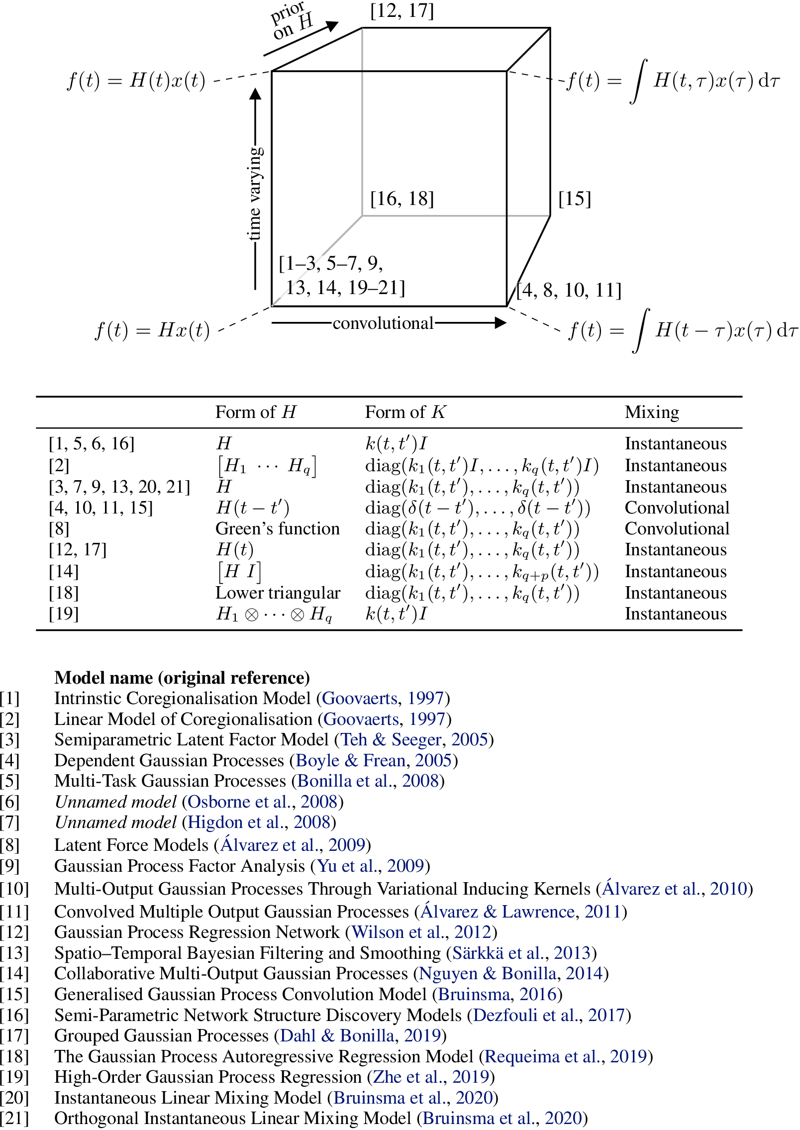Figure 3: Diagram relating several models from the literature to the MMH, based on their properties.

Naturally, these different members of the MMH vary in complexity and each brings their own set of challenges. Particularly, exact inference is computationally expensive or even intractable for many models in the MMH, which requires the use of approximate inference methods such as variational inference (VI), or even Markov Chain Monte Carlo (MCMC). We definitely recommend the reading of the original papers if one is interested in seeing all the clever ways the authors find to perform inference efficiently.

Although the MMH defines a large and powerful family of models, not all multi-output Gaussian process models are covered by it. For example, Deep GPs and its variations are excluded because they transform the latent processes nonlinearly to generate the observations.

Conclusion

In this post we have briefly discussed how to extend regular, single output Gaussian Processes (GP) to multi-output Gaussian Processes (MOGP), and argued that MOGPs are really just single-output GPs after all. We have also introduced the Mixing Model Hierarchy (MMH), which classifies a large number of models from the MOGP literature based on the way they generalise a particular base model, the Instantaneous Linear Mixing Model (ILMM).

In the next post of this series, we are going to discuss the ILMM in more detail and show how some simple assumptions can lead to a much more scalable model, which is applicable to extremely large systems that not even the simplest members of the MMH can tackle in general.

Notes