Using Meta-optimization for Predicting Solutions to Optimal Power Flow

17 Dec 2021

Author: Letif Mones

In a previous blog post, we reviewed how neural networks (NNs) can be used to predict solutions of optimal power flow (OPF) problems. We showed that widely used approaches fall into two major classes: end-to-end and hybrid techniques. In the case of end-to-end (or direct) methods, a NN is applied as a regressor and either the full set or a subset of the optimization variables is predicted based on the grid parameters (typically active and reactive power loads). Hybrid (or indirect) approaches include two steps: in the first step, some of the inputs of OPF are inferred by a NN, and in the second step an OPF optimization is performed with the predicted inputs. This can reduce the computational time by either enhancing convergence to the solution or formulating an equivalent but smaller problem.

Under certain conditions, hybrid techniques provide feasible (and sometimes even optimal) values of the optimization variables of the OPF. Therefore, hybrid approaches constitute an important research direction in the field. However, feasibility and optimality have their price: because of the requirement of solving an actual OPF, hybrid methods can be computationally expensive, especially when compared to end-to-end techniques. In this blog post, we discuss an approach to minimize the total computational time of hybrid methods by applying a meta-objective function that directly measures this computational cost.

Hybrid NN-based methods for predicting OPF solutions

In this post we will focus solely on hybrid NN-based methods. For more detailed theoretical background we suggest reading our earlier blog post.

OPF problems are mathematical optimizations with the following concise and generic form:

\[\begin{equation} \begin{aligned} & \min \limits_{y}\ f(x, y) \\ & \mathrm{s.\ t.} \ \ c_{i}^{\mathrm{E}}(x, y) = 0 \quad i = 1, \dots, n \\ & \quad \; \; \; \; \; c_{j}^{\mathrm{I}}(x, y) \ge 0 \quad j = 1, \dots, m \\ \end{aligned} \label{opt} \end{equation}\]

where \(x\) is the vector of grid parameters and \(y\) is the vector of optimization variables, \(f(x, y)\) is the objective (or cost) function to minimize, subject to equality constraints \(c_{i}^{\mathrm{E}}(x, y) \in \mathcal{C}^{\mathrm{E}}\) and inequality constraints \(c_{j}^{\mathrm{I}}(x, y) \in \mathcal{C}^{\mathrm{I}}\). For convenience we write \(\mathcal{C}^{\mathrm{E}}\) and \(\mathcal{C}^{\mathrm{I}}\) for the sets of equality and inequality constraints, with corresponding cardinalities \(n = \lvert \mathcal{C}^{\mathrm{E}} \rvert\) and \(m = \lvert \mathcal{C}^{\mathrm{I}} \rvert\), respectively.

This optimization problem can be non-linear, non-convex, and even mixed-integer. The most widely used approach to solving it is the interior-point method.^{1 2 3} The interior-point method is based on an iteration, which starts from an initial value of the optimization variables (\(y^{0}\)). At each iteration step, the optimization variables are updated based on the Newton-Raphson method until some convergence criteria have been satisfied.

OPF can be also considered as an operator⁴ that maps the grid parameters (\(x\)) to the optimal value of the optimization variables (\(y^{*}\)). In a more general sense (Figure 1), the objective and constraint functions, as well as the initial value of the optimization variables, are also arguments of this operator and we can write:

\[\begin{equation} \Phi: \Omega \to \mathbb{R}^{n_{y}}: \quad \Phi\left( x, y^{0}, f, \mathcal{C}^{\mathrm{E}}, \mathcal{C}^{\mathrm{I}} \right) = y^{*}, \label{opf-operator} \end{equation}\]

where \(\Omega\) is an abstract set within the values of the operator arguments are allowed to change and \(n_{y}\) is the dimension of the optimization variables.

Hybrid NN-based techniques apply neural networks to predict some arguments of the operator in order to reduce the computational time of running OPF compared to default methods.

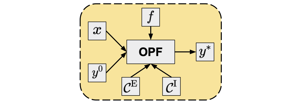Figure 1. OPF as an operator.

Regression-based hybrid methods

Starting the optimization from a specified value of the optimization variables (rather than the default used by a given solver) in the framework of interior-point methods is called warm-start optimization. Directly predicting the optimal values of the optimization variables (end-to-end or direct methods) can result in a sub-optimal or even infeasible point. However, as it is presumably close enough to the solution, it seems to be a reasonable approach to use this predicted value as the starting point of a warm-start optimization. Regression-based indirect techniques follow exactly this route^{5 6}: for a given grid parameter vector \(x_{t}\), a NN is applied to obtain the predicted set-point, \(\hat{y}_{t}^{0} = \mathrm{NN}_{\theta}^{\mathrm{r}}(x_{t})\), where the subscript \(\theta\) denotes all parameters (weights, biases, etc.) of the NN, and the superscript \(\mathrm{r}\) indicates that the NN is used as a regressor. Based on the predicted set-point, a warm-start optimization can be performed:

\[\begin{equation} \begin{aligned} \hat{\Phi}^{\mathrm{red}}(x_{t}) &= \Phi \left( x_{t}, \hat{y}_{t}^{0}, f, \mathcal{C}^{\mathrm{E}}, \mathcal{C}^{\mathrm{I}} \right) \\ &= \Phi \left( x_{t}, \mathrm{NN}_{\theta}^{\mathrm{r}}(x_{t}), f, \mathcal{C}^{\mathrm{E}}, \mathcal{C}^{\mathrm{I}} \right) \\ &= y_{t}^{*}. \end{aligned} \end{equation}\]

Warm-start methods provide an exact (locally) optimal point, as the solution is eventually obtained from an optimization problem identical to the original one.

Training the NN is performed by minimizing the sum (or mean) of some differentiable loss function of the training samples with respect to the NN parameters:

\[\begin{equation} \min \limits_{\theta} \sum \limits_{t=1}^{N_{\mathrm{train}}} L^\mathrm{r} \left(y_{t}^{*}, \hat{y}_{t}^{(0)} \right), \end{equation}\]

where \(N_{\mathrm{train}}\) denotes the number of training samples and \(L^{\mathrm{r}} \left(y_{t}^{*}, \hat{y}_{t}^{(0)} \right)\) is the (regression) loss function between the true and predicted values of the optimal point. Typical loss functions are the (mean) squared error, \(SE \left(y_{t}^{*}, \hat{y}_{t}^{(0)} \right) = \left\| y_{t}^{*} - \hat{y}_{t}^{(0)} \right\|^{2}\), and (mean) absolute error, \(AE \left(y_{t}^{*}, \hat{y}_{t}^{(0)} \right) = \left\| y_{t}^{*} - \hat{y}_{t}^{(0)} \right\|\) functions.

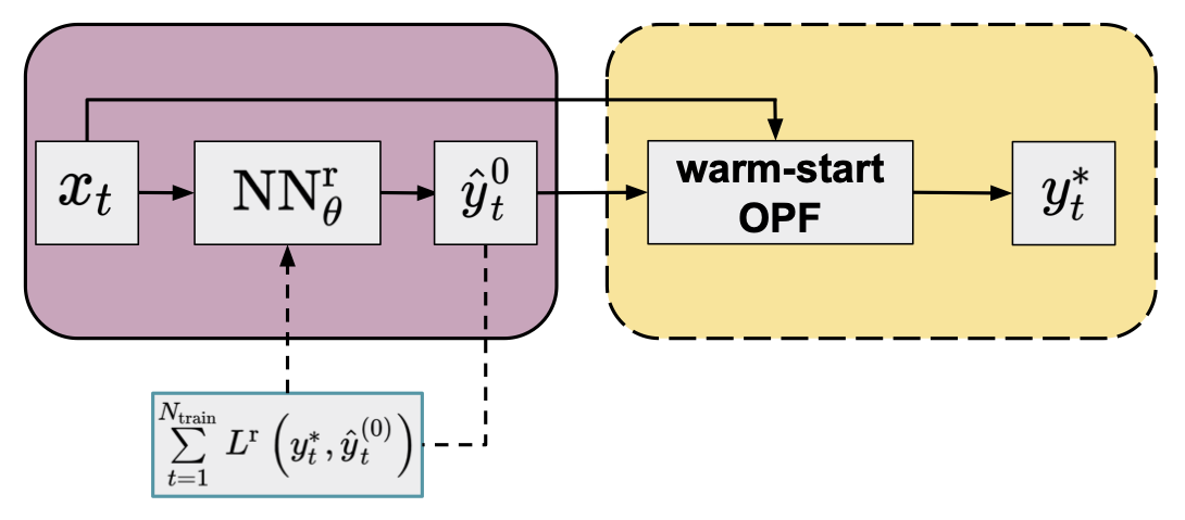Figure 2. Flowchart of the warm-start method (yellow panel) in combination with an NN regressor (purple panel, default arguments of OPF operator are omitted for clarity) trained by minimizing a conventional loss function.

Classification-based hybrid methods

An alternative hybrid approach using a NN classifier (\(\mathrm{NN}_{\theta}^{\mathrm{c}}\)) leverages the observation that only a fraction of all constraints is binding at the optimum^{7 8}, so a reduced OPF problem can be formulated by keeping only the binding constraints. Since this reduced problem still has the same objective function as the original one, the solution should be equivalent to that of the original full problem: \(\Phi \left( x_{t}, y^{0}, f, \mathcal{C}^{\mathrm{E}}, \mathcal{A}_{t} \right) = \Phi \left( x_{t}, y^{0}, f, \mathcal{C}^{\mathrm{E}}, \mathcal{C}^{\mathrm{I}} \right) = y_{t}^{*}\), where \(\mathcal{A}_{t} \subseteq \mathcal{C}^{\mathrm{I}}\) is the active or binding subset of the inequality constraints (also note that \(\mathcal{C}^{\mathrm{E}} \cup \mathcal{A}_{t}\) contains all active constraints defining the specific congestion regime). This suggests a classification formulation in which the grid parameters are used to predict the active set:

\[\begin{equation} \begin{aligned} \hat{\Phi}^{\mathrm{red}}(x_{t}) &= \Phi \left( x_{t}, y^{0}, f, \mathcal{C}^{\mathrm{E}}, \hat{\mathcal{A}}_{t} \right) \\ &= \Phi \left( x_{t}, y^{0}, f, \mathcal{C}^{\mathrm{E}}, \mathrm{NN}_{\theta}^{\mathrm{c}}(x_{t}) \right) \\ &= \hat{y}_{t}^{*}. \end{aligned} \end{equation}\]

Technically, the NN can be used in two ways to predict the active set. One approach is to identify all distinct active sets in the training data and train a multiclass classifier that maps the input to the corresponding active set.⁸ Since the number of active sets increases exponentially with system size, for larger grids it might be better to predict the binding status of each non-trivial constraint by using a binary multi-label classifier.⁹

However, since the classifiers are not perfect, there may be violated constraints not included in the reduced model. One of the most widely used approaches to ensure convergence to an optimal point of the full problem is the iterative feasibility test.^{10 9} The procedure has been widely used by power grid operators and it includes the following steps in combination with a classifier:

1. An initial active set of inequality constraints (\(\hat{\mathcal{A}}_{t}^{(1)}\)) is proposed by the classifier and a solution of the reduced problem is obtained.
2. In each feasibility iteration, \(k = §1, \ldots, K\), the optimal point of the actual reduced problem (\({\hat{y}_{t}^{*}}^{(k)}\)) is validated against the constraints \(\mathcal{C}^{\mathrm{I}}\) of the original full formulation.
3. At each step \(k\), the violated constraints \(\mathcal{N}_{t}^{(k)} \subseteq \mathcal{C}^{\mathrm{I}} \setminus \hat{\mathcal{A}}_{t}^{(k)}\) are added to the set of considered inequality constraints to form the active set of the next iteration: \(\hat{\mathcal{A}}_{t}^{(k+1)} = \hat{\mathcal{A}}_{t}^{(k)} \cup \mathcal{N}_{t}^{(k)}\).
4. The procedure repeats until no violations are found (i.e. \(\mathcal{N}_{t}^{(k)} = \emptyset\)), and the optimal point satisfies all original constraints \(\mathcal{C}^{\mathrm{I}}\). At this point, we have found the optimal point to the full problem (\({\hat{y}_{t}^{*}}^{(k)} = y_{t}^{*}\)).

As the reduced OPF is much cheaper to solve than the full problem, this procedure (if converged in few iterations) can be in theory very efficient, resulting in an optimal solution to the full OPF problem. Obtaining optimal NN parameters is again based on minimizing a loss function of the training data:

\[\begin{equation} \min \limits_{\theta} \sum \limits_{t=1}^{N_{\mathrm{train}}} L^{\mathrm{c}} \left( \mathcal{A}_{t}, \hat{\mathcal{A}}_{t}^{(1)} \right), \end{equation}\]

where \(L^{\mathrm{c}} \left( \mathcal{A}_{t}, \hat{\mathcal{A}}_{t}^{(1)} \right)\) is the classifier loss as a function of the true and predicted active inequality constraints. For instance, for predicting the binding status of each potential constraint, the typical loss function used is the binary cross-entropy: \(BCE \left( \mathcal{A}_{t}, \hat{\mathcal{A}}_{t}^{(1)} \right) = -\frac{1}{m} \sum \limits_{j=1}^{m} c^{(t)}_{j} \log \hat{c}^{(t)}_{j} + \left( 1 - c^{(t)}_{j} \right) \log \left( 1 - \hat{c}^{(t)}_{j} \right)\), where \(c_{j}^{(t)}\) and \(\hat{c}_{j}^{(t)}\) are the true value and predicted probability of the binding status of the \(j\)th inequality constraint.

Figure 3. Flowchart of the iterative feasibility test method (yellow panel) in combination with a NN classifier (purple panel; default arguments of OPF operator are omitted for clarity) trained by minimizing a conventional loss function.

Meta-loss

In the previous sections, we discussed hybrid methods that apply a NN either as a regressor or a classifier to predict starting values of the optimization variables and initial set of binding constraints, respectively, for the subsequent OPF calculations. During the optimization of the NN parameters some regression- or classification-based loss function of the training data is minimized. However, below we will show that these conventional loss functions do not necessarily minimize the most time consuming part of the hybrid techniques, i.e. the computationally expensive OPF step(s). Therefore, we suggest a meta-objective function that directly addresses this computational cost.

Meta-optimization for regression-based hybrid approaches

Conventional supervised regression techniques typically use loss functions based on a distance between the training ground-truth and predicted output value, such as mean squared error or mean absolute error. In general, each dimension of the target variable is treated equally in these loss functions. However, the shape of the Lagrangian landscape of the OPF problem as a function of the optimization variables is far from isotropic¹¹, implying that optimization under such an objective does not necessarily minimize the warm-started OPF solution time. Also, trying to derive initial values for optimization variables using empirical risk minimization techniques does not guarantee feasibility, regardless of the accuracy of the prediction to the ground truth. Interior-point methods start by first moving the system into a feasible region, thereby potentially altering the initial position significantly. Consequently, warm-starting from an infeasible point can be inefficient.

Instead, one can use a meta-loss function that directly measures the computational cost of solving the (warm-started) OPF problem.^{6 9} One measure of the computational cost can be defined by the number of iterations \((N(\hat{y}^{0}_{t}))\) required to reach the optimal solution. Since the warm-started OPF has exactly the same formulation as the original OPF problem, the comparative number of iterations represents the improvement in computational cost. Alternatively, the total CPU time of the warm-started OPF \((T(\hat{y}^{0}_{t}))\) can also be measured, although, unlike the number of iterations, it is not a noise-free measure. Figure 4 presents a flowchart of the procedure for using a NN with parameters determined by minimizing the computational time-based meta-loss function (meta-optimization) on the training set. As this meta-loss is a non-differentiable function with respect to the NN weights, back-propagation cannot be used. As an alternative, one can employ gradient-free optimization techniques.

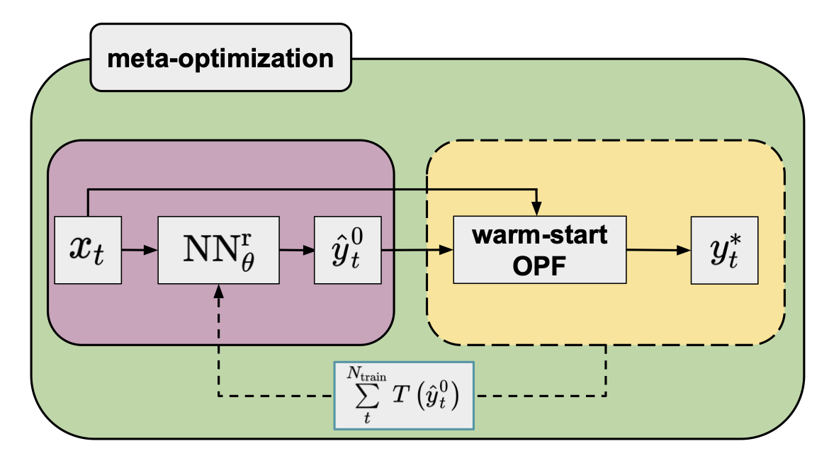Figure 4. Flowchart of the warm-start method (yellow panel) in combination with an NN regressor (purple panel; default arguments of the OPF operator are omitted for clarity) trained by minimizing a meta-loss function that is a sum of the computational time of warm-started OPFs of the training data.

Meta-optimization for classification-based hybrid approaches

In the case of the classification-based hybrid methods, the goal is to find NN weights that minimize the total computational time of the iterative feasibility test. However, minimizing a cross-entropy loss function to obtain such weights is not straightforward. First, the number of cycles in the iterative procedure is much more sensitive to false negative than to false positive predictions of the binding status. Second, different constraints can be more or less important depending on the actual congestion regime and binding status (Figure 5). These suggest the use of a more sophisticated objective function, for instance a weighted cross-entropy with appropriate weights for the corresponding terms. The weights as hyperparameters can then be optimized to achieve an objective that can adapt to the above requirements. However, an alternative objective can be defined as the total computational time of the iterative feasibility test procedure.⁹

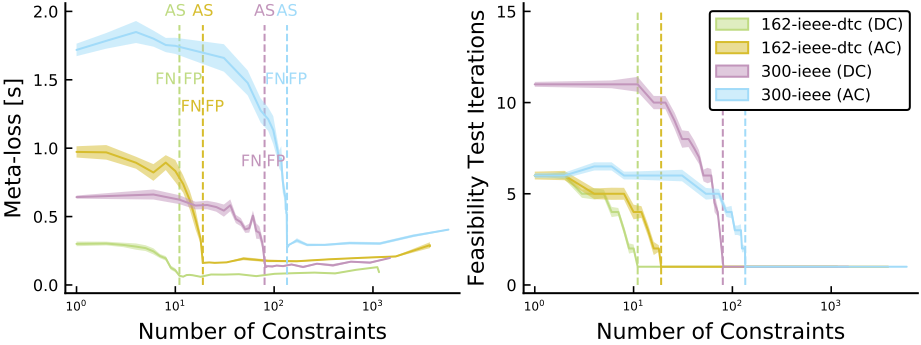Figure 5. Profile of the meta-loss (total computational time) and number of iterations within the iterative feasibility test as functions of the number of constraints for two grids, and a comparison of DC vs. AC formulations. Perfect classifiers with the active set (AS) are indicated by vertical dashed lines, with the false positive (FP) region to the right, and the false negative (FN) region to the left.⁹

The meta-loss objective, therefore, includes the solution time of a sequence of reduced OPF problems. Similarly to the meta-loss defined for the regression approach, it measures the computational cost of obtaining a solution of the full problem and, unlike weighted cross-entropy, it does not require additional hyperparameters to be optimized.

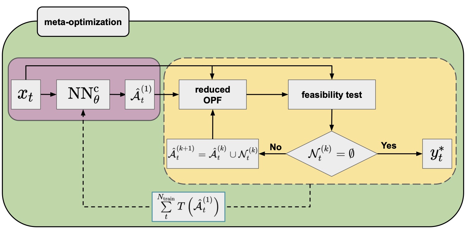Figure 6. Flowchart of the iterative feasibility test method (yellow panel) in combination with an NN classifier (purple panel; default arguments of the OPF operator are omitted for clarity) trained by minimizing a meta-loss function that is a sum of the computational time of the iterative feasibility tests of the training data.

Optimizing the meta-loss function: the particle swarm optimization method

Neither the number of iterations nor the computational time of the subsequent OPF is a differentiable quantity with respect to the applied NNs. Therefore, to obtain optimal NN weights by minimizing the meta-loss, a gradient-free method (i.e. using only the value of the loss function) is required.
The particle swarm optimization was found to be a particularly promising⁹ gradient-free approach for this.

Particle swarm optimization (PSO) is a gradient-free meta-heuristic algorithm inspired by the concept of swarm intelligence that can be found in nature within certain animal groups. The method applies a set of particles (\(N_{\mathrm{p}}\)) and the particle dynamics at each optimization step is influenced by both the individual (best position found by the particle) and collective (best position found among all particles) knowledge. More specifically, for a \(D\) dimensional problem, each particle \(p\) is associated with a velocity \(v^{(p)} \in \mathbb{R}^{D}\) and position \(x^{(p)} \in \mathbb{R}^{D}\) vectors that are randomly initialized at the beginning of the optimization within the corresponding ranges of interest. During the course of the optimization, the velocities and positions are updated and in the \(n\)th iteration, the new vectors are obtained as¹²:

\[\begin{equation} \begin{aligned} v_{n+1}^{(p)} & = \underbrace{\omega_{n} v_{n}^{(p)}}_{\mathrm{inertia}} + \underbrace{c_{1} r_{n} \odot (l_{n}^{(p)} - x_{n}^{(p)})}_{\mathrm{local\ information}} + \underbrace{c_{2} q_{n} \odot (g_{n} - x_{n}^{(p)})}_{\mathrm{global\ information}} \\ x_{n+1}^{(p)} & = x_{n}^{(p)} + v_{n+1}^{(p)}, \end{aligned} \label{eq:pso} \end{equation}\]

where \(\omega_{n}\) is the inertia weight, \(c_{1}\) and \(c_{2}\) are the acceleration coefficients, \(r_{n}\) and \(q_{n}\) are random vectors whose each component is drawn from a uniform distribution within the \([0, 1]\) interval, \(l_{n}^{(p)}\) is the best local position found by particle \(p\) and \(g_{n}\) is the best global position found by all particles together so far, and \(\odot\) denotes the Hadamard (pointwise) product.

As it seems from eq. \ref{eq:pso}, PSO is a fairly simple approach: the particles’ velocity is governed by three terms: inertia, local and global knowledge. The method was originally proposed for global optimization and it can be easily parallelized across the particles.

Numerical experiments

We demonstrate the increased performance of the meta-loss objective compared to conventional loss functions for the classification-based hybrid approach. Three synthetic grids using both DC and AC formulations were investigated using 10k and 1k samples, respectively. The samples were split randomly into training, validation, and test sets containing 70%, 20%, and 10% of the samples, respectively.

A fully connected NN was trained using a conventional and a weighted cross-entropy objective function in combination with a standard gradient-based optimizer (ADAM). As discussed earlier, the meta-loss is much more sensitive to false negative predictions (Figure 5). To reflect this in the weighted cross-entropy expression, we applied weights of 0.25 and 0.75 for the false positive and false negative penalty terms. Then, starting from these optimized NNs, we performed further optimizations, using the meta-loss objective in combination with a PSO optimizer.

Table 1 includes the average computational gains (compared to the full problem) of the different approaches using 10 independent experiments for each. For all cases, the weighted cross-entropy objective outperforms the conventional cross-entropy, indicating the importance of the false negative penalty term. However, optimizing the NNs further by the meta-loss objective significantly improves the computational gain for both cases. For AC-OPF, it brings the gain into the positive regime. For details on how to use a meta-loss function, as well as for further numerical results, we refer to our paper.⁹

Table 1. Average gain with two sided \(95\)% confidence intervals of classification-based hybrid models in combination with meta-optimization using conventional and weighted binary cross-entropy for pre-training the NN.

Case	Gain (%)
	Conventional		Weighted
	Cross-entropy	Meta-loss	Cross-entropy	Meta-loss
DC-OPF
118-ieee	$$\begin{equation*}38.2 \pm 0.8\end{equation*}$$	$$\begin{equation*}42.1 \pm 2.7\end{equation*}$$	$$\begin{equation*}43.0 \pm 0.5\end{equation*}$$	$$\begin{equation*}44.8 \pm 1.2\end{equation*}$$
162-ieee-dtc	$$\begin{equation*}8.9 \pm 0.9\end{equation*}$$	$$\begin{equation*}31.2 \pm 1.3\end{equation*}$$	$$\begin{equation*}21.2 \pm 0.7\end{equation*}$$	$$\begin{equation*}36.9 \pm 1.0\end{equation*}$$
300-ieee	$$\begin{equation*}-47.1 \pm 0.5\end{equation*}$$	$$\begin{equation*}11.8 \pm 5.2\end{equation*}$$	$$\begin{equation*}-10.2 \pm 0.8\end{equation*}$$	$$\begin{equation*}23.2 \pm 1.8\end{equation*}$$
AC-OPF
118-ieee	$$\begin{equation*}-31.7 \pm 1.2\end{equation*}$$	$$\begin{equation*}20.5 \pm 4.2\end{equation*}$$	$$\begin{equation*}-3.8 \pm 2.3\end{equation*}$$	$$\begin{equation*}29.3 \pm 2.0\end{equation*}$$
162-ieee-dtc	$$\begin{equation*}-60.5 \pm 2.7\end{equation*}$$	$$\begin{equation*}8.6 \pm 7.6\end{equation*}$$	$$\begin{equation*}-28.4 \pm 3.0\end{equation*}$$	$$\begin{equation*}23.4 \pm 2.2\end{equation*}$$
300-ieee	$$\begin{equation*}-56.0 \pm 5.8\end{equation*}$$	$$\begin{equation*}5.0 \pm 6.4\end{equation*}$$	$$\begin{equation*}-30.9 \pm 2.2\end{equation*}$$	$$\begin{equation*}15.8 \pm 2.3\end{equation*}$$

Conclusion

NN-based hybrid approaches can guarantee optimal solutions and are therefore a particularly interesting research direction among machine learning assisted OPF models. In this blog post, we argued that the computational cost of the subsequent (warm-start or set of reduced) OPF can be straightforwardly reduced by applying a meta-loss objective. Unlike conventional loss functions that measure some error between the ground truth and the predicted quantities, the meta-loss objective directly addresses the computational time. Since the meta-loss is not a differentiable function of the NN weights, a gradient-free optimization technique, like the particle swarm optimization approach, can be used.

Although significant improvements of the computational cost of OPF can be achieved by applying a meta-loss objective compared to conventional loss functions, in practice these gains are still far from desirable (i.e. the total computational cost should be a fraction of that of the original OPF problem).⁹

In a subsequent blog post, we will discuss how neural networks can be utilized in a more efficient way to obtain optimal OPF solutions.

---