This post is a short note on the notorious Y combinator.
No, not that company, but the computer sciency objects that looks like this:
\[\label{eq:Y-combinator}
Y = \lambda\, f : (\lambda\, x : f\,(x\, x))\, (\lambda\, x : f\,(x\, x)).\]
Don’t worry if that looks complicated; we’ll get down to some examples and the nitty gritty details in just a second.
But first, what even is this Y combinator thing?
Simply put, the Y combinator is a higher-order function \(Y\) that can be used to define recursive functions in languages that don’t support recursion.
Cool!
For readers unfamiliar with the above notation, the right-hand side of Equation \eqref{eq:Y-combinator} is a lambda term, which is a valid expression in lambda calculus:
\(x\), a variable, is a lambda term;
if \(t\) is a lambda term, then the anonymous function \(\lambda\, x : t\) is a lambda term;
if \(s\) and \(t\) are lambda terms, then \(s\, t\) is a lambda term, which should be interpreted as \(s\) applied with argument \(t\); and
nothing else is a lambda term.
For example, if we apply \(\lambda\, x : y\,x\) to \(z\), we find
\[\label{eq:example}
(\lambda\, x : y\,x)\, z = y\,z.\]
Although the notation in Equation \eqref{eq:example} suggests multiplication, note that everything is function application, because really that’s all there is in lambda calculus.
In words, if \(n\) is zero, return \(1\); otherwise, multiply \(n\) with \(\code{fact}(n-1)\).
Equation \eqref{eq:fact-recursive} would be a valid expression if lambda calculus would allow us to use \(\code{fact}\) in the definition of \(\code{fact}\).
Unfortunately, it doesn’t.
Tricky.
Let’s replace the inner \(\code{fact}\) by a variable \(f\):
Now, crucially, the Y combinator \(Y\) is precisely designed to construct \(\code{fact}\) from \(\code{fact}'\):
\[Y\, \code{fact}' = \code{fact}.\]
To see this, let’s denote \(\code{fact2}=Y\,\code{fact}'\) and verify that \(\code{fact2}\) indeed equals \(\code{fact}\):
\begin{align}
\code{fact2}
&= Y\, \code{fact}’ \newline
&= (\lambda\, f : (\lambda\, x : f\,(x\, x))\, (\lambda\, x : f\,(x\, x)))\, \code{fact}’ \newline
&= (\lambda\, x : \code{fact}’\,(x\, x) )\, (\lambda\, x : \code{fact}’\,(x\, x)) \label{eq:step-1} \newline
&= \code{fact}’\, ((\lambda\, x : \code{fact}’\, (x\, x))\,(\lambda\, x : \code{fact}’\, (x\, x))) \label{eq:step-2} \newline
&= \code{fact}’\, (Y\, \code{fact}’) \newline
&= \code{fact}’\, \code{fact2},
\end{align}
which is exactly what we’re looking for, because the first argument to \(\code{fact}'\) should be the actual factorial function, \(\code{fact2}\) in this case.
Neat!
We hence see that \(Y\) can indeed be used to define recursive functions in languages that don’t support recursion.
Where does this magic come from, you say?
Sit tight, because that’s up next!
Deriving the Y Combinator
This section introduces a simple trick that can be used to derive Equation \eqref{eq:Y-combinator}.
We also show how this trick can be used to derive analogues of the Y combinator that implement mutual recursion in languages that don’t even support simple recursion.
Again, let’s start out by considering a recursive function:
\[f = \lambda\, x:g[f, x]\]
where \(g\) is some lambda term that depends on \(f\) and \(x\).
As we discussed before, such a definition is not allowed.
However, pulling out \(f\),
\[\label{eq:fixed-point}
f = \underbrace{(\lambda \, f' :\lambda\, x:g[f', x])}_{h}\,\, f = h\, f.\]
we do find that \(f\) is a fixed point of \(h\): \(f\) is invariant under applications of \(h\).
Now—and this is the trick—suppose that \(f\) is the result of a function \(\hat{f}\) applied to itself: \(f=\hat{f}\,\hat{f}\).
Then Equation \eqref{eq:fixed-point} becomes
\[f
= (\lambda\, h': (\lambda\,x:h'\,(x\,x))\,(\lambda\,x:h'\,(x\,x)))\, h
= Y\, h,\]
where suddenly a wild Y combinator has appeared.
The above derivation shows that \(Y\) is a fixed-point combinator.
Passed some function \(h\), \(Y\,h\) gives a fixed point of \(h\):
\(f = Y\,h\) satisfies \(f = h\,f\).
Pushing it even further, consider two functions that depend on each other:
\begin{align}
f &= \lambda\,x:k_f[x, f, g], &
g &= \lambda\,x:k_g[x, f, g]
\end{align}
where \(k_f\) and \(k_g\) are lambda terms that depend on \(x\), \(f\), and \(g\).
This is foul play, as we know.
We proceed as before and pull out \(f\) and \(g\):
\begin{align}
f
= \underbrace{
(\lambda\,f’:\lambda\,g’:\lambda\,x:k_f[x, f’, g’])
}_{h_f} \,\, f\, g
= h_f\, f\, g
\end{align}
\begin{align}
g
= \underbrace{
(\lambda\,f’:\lambda\,g’:\lambda\,x:k_g[x, f’, g’])
}_{h_g} \,\, f\, g
= h_g\, f\, g.
\end{align}
Now—here’s that trick again—let \(f = \hat{f}\,\hat{f}\,\hat{g}\) and \(g = \hat{g}\,\hat{f}\,\hat{g}\).1
Then
Dang, laborious, but that worked.
And thus we have derived two analogues \(Y_f\) and \(Y_g\) of the Y combinator that implement mutual recursion in languages that don’t even support simple recursion.
Implementing the Y Combinator in Python
Well, that’s cool and all, but let’s see whether this Y combinator thing actually works.
Consider the following nearly 1-to-1 translation of \(Y\) and \(\code{fact}'\) to Python:
Eh?
What’s going?
Let’s, for closer inspection, once more write down \(Y\):
\[Y = \lambda\, f: (\lambda\, x : f\,(x\, x))\, (\lambda\, x : f\,(x\, x)).\]
After \(f\) is passed to \(Y\), \((\lambda\, x : f\,(x\, x))\) is passed to \((\lambda\, x : f\,(x\, x))\); which then evaluates \(x\, x\), which passes \((\lambda\, x : f\,(x\, x))\) to \((\lambda\, x : f\,(x\, x))\); which then again evaluates \(x\, x\), which again passes \((\lambda\, x : f\,(x\, x))\) to \((\lambda\, x : f\,(x\, x))\); ad infinitum.
Written down differently, evaluation of \(Y\, f\, x\) yields
\[Y\, f\, x
= (Y\, f)\, x
= (Y\, (Y\, f))\, x
= (Y\, (Y\, (Y\, f)))\, x
= (Y\, (Y\, (Y\, (Y\, f))))\, x
= \ldots,\]
which goes on indefinitely.
Consequently, \(Y\, f\) will not evaluate in finite time, and this is the cause of the RecursionError.
But we can fix this, and quite simply so: only allow the recursion—the \(x\,x\) bit—to happen when it’s passed an argument; in other words, replace
To recapitulate, the Y combinator is a higher-order function that can be used to define recursion—and even mutual recursion—in languages that don’t support recursion.
One way of deriving \(Y\) is to assume that the recursive function under consideration \(f\) is the result of some other function \(\hat{f}\) applied to itself:
\(f = \hat{f}\,\hat{f}\);
after some simple manipulation, the result can then be determined by inspection.
Although \(Y\) can indeed be used to define recursive functions, it cannot be applied literally in a contemporary programming language; recursion errors might then occur.
Fortunately, this can be fixed simply by letting the recursion in \(Y\) happen when needed—that is, lazily.
Do you see why this is the appropriate generalisation of letting \(f=\hat{f}\,\hat{f}\)? ↩
In the US, discussions regarding coal tend to be divisive, and are often driven more by politics than data. In this post, we will take an exploratory dive into detailed public data related to electricity generation from coal, and show how this can be used to better understand these systems and the changes they have been undergoing in recent years.
We will look specifically at aspects related to the life cycle of coal, from its origin in coal mines, to its shipments within and between regions, and on to its final use in coal-fired power plants. We will also focus on coal use for electricity generation, as the US electric power sector is responsible for about 90% of overall consumption of coal.
The raw data is available in a JSON format, and is very detailed, with information on shipments from specific coal mines to power plants, and also on the operating statistics of power plants.
The animation below shows the yearly amount of coal produced, both at the level of individual mines, and also aggregated statistics for total mine production per state.
From this, one can see that the mines tend to be locally concentrated based on the various coal basins, and also that the amount of production is by no means evenly distributed.
Yearly coal production for electricity usage, shown at both mine and state level.
As someone who grew up in the US, this map challenges the common mythology I often heard about Appalachia and coal mining, and assumptions about states such as West Virginia being dominant producers.
While Appalachia was a primary source of coal historically, it has been far eclipsed by Wyoming’s Powder River Basin.
The Powder River Basin is composed of surface mines with giant coal seams as shown below.
This region produces around 42% of all coal in the US1, with the North Antelope Rochelle Mine alone providing 12% of total US production in 20162.
This single mine produces more coal than West Virginia, the second largest coal mining state.
The animated map below by the Google Earth Engine Timelapse shows the enormous geographic scale of the Power River Basin mines, along with their historical growth over 32 years of satellite imagery.
Over time, one can see new areas being dug out with land restoration efforts following shortly behind.
The EIA data on coal shipments has incredible resolution, and one can find information about quarterly shipments between individual mines and power plants.
For each of these there is information about the type of coal, ash content, heat content, price, quantity, and sulfur content.
The sulfur content of coal is a concern due to SO2 pollution resulting from coal combustion, which can lead to problems such as acid rain, respiratory problems, and atmospheric haze.
While high sulfur content does not necessarily translate into high SO2 emissions due to desulfurization technology used by power plants to reduce emissions3, the process of desulfurization is an economic cost rather than a benefit, and examining sulfur content can at a minimum give indications related to the economics of coal prices.
The plot below gives an overview of how the coal produced each year differs in the amount of sulfur content.
To construct the plot, we did the following:
Per year, sort all coal shipments from those with the highest percentage of sulfur to those with the lowest.
Using this order, calculate the cumulative quantity.
The last value is the total amount of coal produced in the US in that year.
A useful feature of this type of plot is that the area under the curve is the total amount of sulfur contained in coal shipments that year.
Instead of reducing the yearly amount of sulfur to a single number, this plot shows how it is distributed based on the properties of the coal shipped.
Profile of coal sulfur content.
For reference, we use 2008 (in blue) as a baseline since that is the first year in the EIA data.
As the animation progresses, we can see that total coal production peaks in 2010, before steadily decreasing to levels below 2008.
By examining the differences between the two curves, we can see where increases and decreases in sulfur from different types of coal have occurred.
For example, on the left side of the plot, the gray areas show increased amounts of sulfur from coal that is high in sulfur.
Later in the animation, we see light blue areas, representing decreased amounts of sulfur from low-sulfur coal (and less coal production overall).
By subtracting the size of the light blue areas from the gray areas, we can calculate the overall change in sulfur, relative to 2008.
As described further below in this post, electricity generation from coal has decreased, although it has been observed that SO2 emissions have fallen quicker than the decrease in generation, in part due to more stringent desulfurization requirements between 2015 and 2016.
The increased production of high-sulfur coal shown in the plot suggests an economic tradeoff, which would be interesting to explore with a more detailed analysis.
For example, while low-sulfur coal commands a higher price, one could also choose high-sulfur coal, but then be faced with the costs of operating the required desulfurization technologies.
Transport
After looking at where coal is produced and some of its properties, we will now examine how much is shipped between different regions.
To visualize this, we use an animated Chord Diagram, using code adapted from an example showing international migrations.
This technique allows us to visually organize the shipments between diverse regions, with the width of the lines representing the size of the shipments in millions of tons.
The axes show the total amount of coal produced and consumed within that year.
Arrows looping back to the same region indicate coal produced and consumed in the same region.
To prevent the visualization from being overly cluttered, we group the US states based on US Census Divisions, with the abbreviations for states in each division indicated.
Yearly coal flows between different US Census Divisions.
In the three divisions at the top of the plot (West North Central, West South Central, and East North Central), the majority of coal is sourced from states in the Mountain division.
The locations of the top five US coal producing states on the plot are indicated below.
This list uses statistics from the EIA for 2016, and includes the total amount of production in megatons, along with their percent contribution to overall US production:
Wyoming: 297.2 MT (41%) - Mountain (bottom)
West Virginia: 79.8 MT (11%) - South Atlantic (left)
Illinois: 43.4 MT (6%) - East North Central (top right)
Kentucky: 42.9 MT (6%) - East South Central (right, above middle)
Overall, coal shipments have been steadily decreasing since a peak around 2010.
Most of the different regions are not self-sufficient, with shipments between regions being common.
Only Mountain is self-sufficient, and it also serves as the dominant supplier in other regions as well.
Looking a bit deeper, checking the annual coal production statistics for the Powder River Basin reveals that with between 313 and 495 MT of annual shipments, it’s the single area responsible for the vast majority of coal shipments originating from Mountain.
Coal Consumption
We now look at what happens to the coal once it’s used for electricity generation, and also put this in context of total electricity generation from all fuel sources.
For this we use the bulk electricity data, specifically the plant level data which can be browsed online.
This data contains monthly information on each power plant, with statistics on the fuel types, amount of electricity generation, and fuel consumed.
While this does not directly document CO2 emissions, we can still estimate them from the available data.
We know how much heat is released from burning fossil fuels at the plant on a monthly basis, in millions of BTUs (MMBTU).
This information can be multiplied by emissions factors from the US EPA that are estimates of how many kilograms of CO2 are emitted for every MMBTU of combusted fuel.
This step tells us how many kilograms of CO2 are emitted on a monthly basis.
By dividing this number of the amount of electricity generation, we then get the CO2 emissions intensity in the form of \(\frac{kg\ CO_2}{MWh}\).
In the plot below, we use the same approach as that in the sulfur content plot above:
Yearly generation is sorted from most CO2 intensive (old coal plants) to the least intensive (renewables).
Using this sorting, the cumulative total generation is calculated.
The area under the curve represents the total CO2 emissions for that year.
Here 2001 is used as the reference year.
Vertical dashed lines are added to indicate total generation for that year, as nuclear and renewables have zero emissions and their generation contributions would not be visible otherwise on the plot.
Also, the y axis is clipped at 1500 kg CO2/MWh to reduce the vertical scale shown.
The plants with higher values can be older, less efficient power plants, or plants that have been completely shut down and need to consume extra fuel to bring the equipment back up to operating temperatures.
Yearly profiles of US electricity generation by carbon intensity.
From the plot we can see that the amount of generation peaked around 2007 and has been roughly stable since then.
While some increases in total emissions occurred after 2001, by looking at 2016, we see that generation from fossil fuels is at the same level as it was in 2001. We can also see two horizontal “shelves”, with the lower one around 400 kg CO2/MWh corresponding to generation from natural gas, and the upper one at 900 kg CO2/MWh corresponding to generation from coal4.
In 2016, these shelves are quite visible, and the light gray area represents a large amount of emissions that were reduced by switching from coal to natural gas.
Overall it’s clear that the US has been steadily decarbonizing the electricity sector.
Another view is shown in the plot below which examines how much of electricity generation is responsible for how much of total CO2 emissions.
The motivation for this is that if you find that 90% of CO2 emissions are from 10% of your electricity generation, then large reductions in CO2 emissions can be achieved by changing only a small fraction of the existing infrastructure.
This plot uses a similar approach as the previous ones, with the following steps:
Sort electricity generation per year, from highest CO2 intensity to lowest.
Calculate total generation and CO2 emissions per year.
Calculate cumulative generation and CO2 emissions per year.
Divide these cumulative totals by the yearly totals to get cumulative percentages.
Starting at 2001, this shows that 27% of electricity generation was from nuclear and renewables, with the remaining 73% from fossil fuels.
Over time, more renewables (such as large amounts of installed wind capacity), more efficient power plants, and a switch from coal to natural gas have pushed this curve to the left and steepened the slope.
As of 2016, 75% of CO2 emissions come from only 35% of electricity generation, with half of CO2 coming from just 21%.
Percent of CO2 emissions coming from percent of electricity generation.
Conclusions
In the above analysis and discussion we looked at only a small subset of what is available in the open data published by the EIA, using a couple of techniques that can help make sense of a deluge of raw data, and tell stories that are not necessarily obvious.
Already it is clear that the US is undergoing a large energy transition with a shift towards more natural gas and renewables.
As this transition continues to unfold, data such as that published by the EIA will be quite important as we make sense of the resulting environmental and economic impacts.
This could be more systematically investigated by linking the power plant identifiers in the coal shipments with the US EPA’s Emissions & Generation Resource Integrated Database (eGRID) data, which contains information about actual SO2 emissions from power plants. This would allow us to do a sulfur mass balance to determine how much sulfur arrives from coal, how much sulfur in the form of SO2 leaves into the atmosphere, and how much sulfur is removed in the scrubbing process. ↩
Higher values for CO2/MWh can be found in literature, especially if life cycle aspects such as emissions from coal mining, transportation, plant operation, etc. are included. The calculations here are only narrowly focused on the combustion of the fuel and the conversion of heat energy into electrical energy. ↩
With the alpha release of version 0.7, Julia has simplified its iteration interface.
This was a huge undertaking which mostly fell to the prolific Keno Fischer, who wrote an entirely new optimizer for the language to accomplish it!
As the most active maintainer of the IterTools package, I decided to spend a week rewriting its iterators for the new interface.
I’d like to share that experience with you to introduce the new interface and assist in transitioning to Julia 0.7.
Iteration in Julia 0.6
Previously, Julia’s iteration interface consisted of three methods: start, next, and done.
A good way to demonstrate how these work together is to show the transformation from a for loop to the equivalent while loop using those functions. I’ve taken this from the Julia Interfaces documentation, written by Matt Bauman and others.
Notice that our EveryNth struct is immutable and we never mutate the state information.
As an aside, the length and eltype method definitions are not necessary.
Instead, we could use the IteratorSize and IteratorEltype traits to say that we don’t implement those functions and Julia’s Base functions will not try to call them when iterating.
collect is notable for specializing on both of these traits to provide optimizations for different kinds of iterators.
Iteration in Julia 0.7
In Julia 0.7, the iteration interface is now just one function: iterate.
The while loop above would now be written as:
The iterate function has two methods.
The first is called once, to begin iteration (like the old start) and also perform the first iteration step.
The second is called repeatedly to iterate, like next in Julia 0.6.
In our iterate function we define a default value for state which is used when iterate is called with one argument. 1
This is already less code than the old interface required, but we can reduce it further using another new feature of Julia 0.7.
function Base.iterate(it::EveryNth,(el,i)=(it.start,0))returni>=it.length?nothing:(el,(el+it.n,i+1))end
I personally prefer verbosity when it increases readability, but some people prefer shorter code, and that’s easier than ever to achieve.
A Note on Compatibility
To assist with transitioning between versions, Julia 0.7 includes fallback definitions of iterate which call start, next, and done.
If you want code to work on both 0.6 and 0.7, I recommend keeping your iterators defined in those terms, as there isn’t a good way to use the iterate interface on Julia 0.6.
Julia 1.0 will remove those fallback definitions and all usage of the old iteration interface.
Common Strategies
The above example was constructed to be as straightforward as possible, but not all iteration is that easy to express.
Luckily, the new interface was designed to assist with situations which were previously difficult or inefficient, and in some cases (like the EveryNth example) reduces the amount of code necessary.
While updatingIterTools.jl, I came across a few patterns which repeatedly proved useful.
Wrapping Another Iterable
In many cases, the iterable we want to create is a transformation applied to a caller-supplied iterable.
Many of the useful patterns apply specifically to this situation.
Early Return
When wrapping an iterable, we usually want to terminate when the wrapped iterable terminates, i.e., return nothing when the wrapped call to iterate returns nothing.
If the call to iterate doesn’t return nothing, we want to apply some operations before returning.
This pattern was common and simple enough to justify a macro which in IterTools I’ve called @ifsomething2:
Conveniently (since it would otherwise error), the value returned from iterate will only be unpacked if it’s not nothing.
Slurping and Splatting
The iteration interface requires two methods of iterate, but it’s handy to use default arguments1 to only write out one function.
However, sometimes there is no clear initial value for state, e.g., if it requires you to start iterating over the wrapped iterable.
In this case it’s helpful to use “slurping” and “splatting”3 to refer to either zero or one function argument—the presence or absence of the state argument.
A simple example is the TakeNth iterator from IterTools.jl.
Its implementation of the iterate function looks like this:
function iterate(it::TakeNth,state...)xs_iter=nothingfori=1:it.intervalxs_iter=@ifsomethingiterate(it.xs,state...)state=Base.tail(xs_iter)endreturnxs_iterend
When you first call iterate(::TakeNth), state starts out as an empty tuple.
Splatting this empty tuple into iterate produces the call iterate(it.xs).
In all further calls, the actual state returned from iterating over the wrapped iterable will be wrapped in a 1-tuple, and unwrapped in each call.
One of the other tools we use here is the unexported function Base.tail(::Tuple).
This function performs the equivalent of slurping on tuples, or xs_iter[2:end].
No matter the size of the input tuple, it will always return at least an empty tuple.
This is especially useful in the next, slightly more complicated example.
For TakeNth, we were only passing around the wrapped iterable’s state, but sometimes we need to carry some state of our own as well.
For the TakeStrict iterator from IterTools.jl we want to iterate over exactly n elements from the wrapped iterable, so we need to carry a counter as well.
function iterate(it::TakeStrict,state=(it.n,))n,xs_state=first(state),Base.tail(state)n<=0&&returnnothingxs_iter=iterate(it.xs,xs_state...)ifxs_iter===nothingthrow(ArgumentError("In takestrict(xs, n), xs had fewer than n items to take."))endv,xs_state=xs_iterreturnv,(n-1,xs_state)end
Here we use Base.tail to slurp the rest of the input after our counter, so xs_state is either an empty tuple (on the initial iterate call) or a 1-tuple containing the state for the wrapped iterable.
Look-ahead Iterators
Occasionally we may want to write an iterable that requires advancing the wrapped iterable before returning a value, such as some kind of generic Fibonnaci iterator, or the simplest example, a “peekable” iterator that can look ahead to the next value.
This exists in IterTools.jl as PeekIter.
function iterate(pit::PeekIter,state=iterate(pit.it))val,it_state=@ifsomethingstatereturn(val,iterate(pit.it,it_state))end
In this case, the work needed for the initial iterate call is just a superset of the regular iterate call, so it’s very simple to implement.
In general, the code for look-ahead iterators is just as easy to write in Julia 0.7, but usually more compact.
Piecewise Development Approach
Having to write many new iterate methods led me to discover some helpful strategies for writing iterate methods when unsure of the best approach.
The most helpful thing I did was to write the two-argument method for iterate first, then write the one-argument method, then try to simplify them into a single method.
Remember that the one-argument method is a combination of the start and next methods from the old iteration interface.
I also realized that it was sometimes easier to apply patterns like the ones above in order to translate from the old to the new iteration interface without attempting to understand the initial version completely.
Let’s look at one of the more complicated iterators in IterTools.jl: Partition.
Something that immediately jumps out about the original is this pattern:
ifdone(it.xs,s)breakend(x,s)=next(it.xs,s)
If there are more items, this advances the wrapped iterable, otherwise it breaks out of the surrounding loop.
In the new interface this requires just one call instead of two:
Then this pattern can be applied by rote wherever it appears.
Applying this and writing two iterate methods results in this4:
function iterate(it::Partition{I,N},state)where{I,N}(xs_state,result)=state# this @ifsomething call handles the 0.6 situation# where `done` is always called before `next`result[end],xs_state=@ifsomethingiterate(it.xs,xs_state)p=similar(result)overlap=max(0,N-it.step)p[1:overlap].=result[it.step.+(1:overlap)]# when step > n, skip over some elementsforiin1:max(0,it.step-N)xs_iter=iterate(it.xs,xs_state)xs_iter===nothing&&break_,xs_state=xs_iterendforiin(overlap+1):(N-1)xs_iter=iterate(it.xs,xs_state)xs_iter===nothing&&breakp[i],xs_state=xs_iterendreturn(tuple(result...),(xs_state,p))endfunction iterate(it::Partition{I,N})where{I,N}result=Vector{eltype(I)}(undef,N)result[1],xs_state=@ifsomethingiterate(it.xs)foriin2:(N-1)result[i],xs_state=@ifsomethingiterate(it.xs,xs_state)endreturniterate(it,(xs_state,result))end
This works for almost every case, except when N == 1!
In that case, we do need to start with iterate(it.xs), but we have to return the first item before calling iterate again, so we have to skip the first iteration in the two-argument method.
It would be nice to have the methods be this simple chain, but it looks like we need to combine them.
Previously, we’ve been able to come up with a sensible default state (or a tuple we can splat) for the combined method.
We can’t5 do that here, as we need to have conditional behaviour for both cases.
Luckily, we can add nothing as a sentinel and Julia will compile the check away.
Making this change results in the version which appears in IterTool 1.0:
function iterate(it::Partition{I,N},state=nothing)where{I,N}ifstate===nothingresult=Vector{eltype(I)}(undef,N)result[1],xs_state=@ifsomethingiterate(it.xs)foriin2:Nresult[i],xs_state=@ifsomethingiterate(it.xs,xs_state)endelse(xs_state,result)=stateresult[end],xs_state=@ifsomethingiterate(it.xs,xs_state)endp=similar(result)overlap=max(0,N-it.step)p[1:overlap].=result[it.step.+(1:overlap)]# when step > n, skip over some elementsforiin1:max(0,it.step-N)xs_iter=iterate(it.xs,xs_state)xs_iter===nothing&&break_,xs_state=xs_iterendforiin(overlap+1):(N-1)xs_iter=iterate(it.xs,xs_state)xs_iter===nothing&&breakp[i],xs_state=xs_iterendreturn(tuple(result...)::eltype(Partition{I,N}),(xs_state,p))end
Conclusion
These are the techniques that helped me in my work, but I’d like to hear about more!
I’m also curious which patterns improve or harm performance and why.
IterTools will definitely accept pull requests, and I’m interested in feedback on Slack and Discourse.
In Julia, this actually defines two methods of iterate, as described in the Julia docs. ↩↩2
Slurping refers to how using args... in a function definition “slurps” up the trailing arguments, and splatting is the inverse operation. The Julia docs say more on this. ↩
All other changes here are renaming or respelling something that appears in the original, for clarity’s sake. ↩
We could, but we’d need to do something different depending on the length of the tuple, which would add another conditional check in addition to the splatting. ↩
In the first part, we discussed the motivation and model behind SyntheticGrids.jl. In this post we show how to use it.
To use SyntheticGrids.jl, Julia 0.6.1 or newer is required. Once Julia is properly installed, the package can be installed via
julia>Pkg.add("SyntheticGrids")
This should take care of all dependencies. In order to check if the package has been properly installed, use
julia>Pkg.test("SyntheticGrids")
A (very) simple test example
As an introduction to the package, we start by automatically generating a small, but complete grid.
julia>usingSyntheticGridsjulia>grid=Grid(false);
This command generates a complete grid corresponding to the region contained in the box defined by latitude [33, 35] and longitude [-95, -93] (default values). It automatically places loads and generators and builds the transmission line network (we will soon see how to do each of these steps manually). Here, false determines that substations will not be created. Note the addition of the semicolon, ;, at the end of the command. This has just cosmetic effect in suppressing the printing of the resulting object in the REPL. Even a small grid object corresponds to a reasonably large amount of data.
A Grid object has several attributes that can be inspected. First, let’s look at the buses:
We see that our grid has a total of 137 buses (see Figure 2 for a visualisation of the result). The first is a load bus (LoadBus). The values of the attributes connected_to and connections are not explicitly printed. However, the printing of (...) indicates that those sets have been populated (otherwise, they would be printed as ()).
Visualisation of two grids generated using the procedure described here. Notice that both present the same bus locations, as their placement is entirely deterministic. The transmission line topology however is different in each case, as it is generated through an stochastic process. Note that the generated grids are non-planar.
The last bus of the list corresponds to a generator (GenBus). One important thing to notice here is that it contains an attribute called gens, which is an array of Generator-type objects. GenBuses represent power plants, which may (or may not, as is the case here) contain several different generating units. These individual generating units are stored within the gens attribute.
There are 167 transmission lines in our grid. By looking at the first one, we see that they are defined by a tuple of Bus-type objects (here both are LoadBuses), by an impedance value (here taken as Real, since the package has been developed with DC OPF in mind), and a current carrying capacity value.
The adjacency matrix of the system can also be easily accessed:
Notice that one of the attributes has been automatically initialised. That corresponds to the seed which will be used for all stochastic steps. Control over the seed value gives us control over reproducibility. Conversely, that value could have been specified via grid = Grid(seed).
Now let’s place the load buses. We could do this by specifying latitude and longitude limits (e.g.: place_loads_from_zips!(grid; latlim = (30, 35), longlim = (-99, -90))), but let’s look at a more general way of doing this. We can define any function that receives a tuple containing a latitude–longitude pair and returns true if within the desired region and false otherwise:
Here, my_region defines a circle (in latitude-longitude space) of radius r around the point (33, -95). Any zip code within that region is added to the grid (to a total of 3287) as a load bus. The same can be done for the generators:
Once all buses are in place, it is time to connect them with transmission lines. This can be done via a single function (this step can take some time for larger grids):
This function goes through the stochastic process of creating the system’s adjacency matrix, but it does not create the actual TransLine objects (hence the zero length). That is done via the create_lines! function. Also note that connect! has several parameters for which we adopted default values. For a description of those, see ? connect.
Before we create the lines, it is interesting to revisit adding new buses. Now that we have created the adjacency matrix for the network, we have two options when adding a new bus: either we redo the connect! step in order to incorporate the new bus in the grid, or we simply extend the adjacency matrix to include the new bus (which won’t have any connections). This is controlled by the reconnect keyword argument that can be passed to add_bus!. In the former case, one uses reconnect = false (the default option); connections can always be manually added by editing the adjacency matrix (and the connected_to fields of the involved buses).
Once the adjacency matrix is ready, TransLine objects are created by invoking the create_lines! function:
We have generated the connection topology with transmission line objects. Finally, we may want to coarse-grain the grid. This is done via the cluster! function, which receives as arguments the number of each type of cluster: load, both load and generation or pure generation. This step may also take a little while for large grids.
At this point, the whole grid has been generated. If you wish to save it, the functions save and load_grid are available. Please note that the floating-point representation of numbers may lead to infinitesimal changes to the values when saving and reloading a grid. Besides precision issues, they should be equivalent.
The generated grid can easily be exported to pandapower in order to carry out powerflow studies. The option to export to PowerModels.jl should be added soon.
Hopefully, this post helped as a first introduction to the SyntheticGrids.jl package. There are more functions which have not been mentioned here; the interested reader should refer to the full documentation for a complete list of methods. This is an ongoing project, and, as such, several changes and additions might still happen. The most up-to-date version can always be found at Github.
It should come as no surprise that electricity plays a vital role in many aspects of modern life. From reading this article, to running essential hospital equipment, or powering your brand-new Tesla, many things that we take for granted would not be possible without the generation and transmission of electrical power. This is only possible due to extensive power grids, which connect power producers with consumers through a very complex network of towers, transmission lines, transformers etc. Needless to say, it is important to understand the peculiarities of these systems in order to avoid large scale blackouts, or your toaster burning out due to a fluctuation in the current.
Power grid research requires testing in realistic, large-scale, electric networks. Real power grids may have tens of thousands of nodes (also called buses), interconnected by multiple power lines each, spanning hundreds of thousands of square kilometers. In light of security concerns, most information on these power grids is considered sensitive and is not available to the general public or to most researchers. This has led to most power transmission studies being done using only a few publicly available test grids 1, 2. These test grids tend to be too small to capture the complexity of real grids, severely limiting the practical applications of such research. With this in mind, there has recently been an effort in developing methods for building realistic synthetic grids, based only on publicly available information. These synthetic grids are based on real power grids and present analogous statistical properties—such as the geographic distribution of load and generation, total load, and generator types—while not actually exposing potentially sensitive information about a real grid.
The pioneers in treating power grids as networks were Watts and Strogatz3, when they pointed out that electric grids share similarities with small-world networks: networks that are highly clustered, but exhibit small characteristic path lengths due to a few individual nodes being directly connected to distant nodes (see Figure 1). This type of network is very useful in explaining social networks— see six degrees of Kevin Bacon—but, despite similarities, power grids differ from small-world networks 4,5. If you are looking for an extensive list of studies on power grids, Pagani and Aiello 6 is a good place to start.
Some examples of different network topologies containing 20 nodes and 40 edges. (a) Small-world; (b) random; (c) scale-free (exponent 2). For more details, see Watts and Strogatz3.
In order to study the dynamic properties of electric grids, some research has adopted simplified topologies, such as tree structures 7 or ring structures 8, which may fail to capture relevant aspects of the system. Efforts to build complete and realistic synthetic grids are a much more recent phenomenon. The effort of two teams is particularly relevant for this post, namely, Overbye’s team 9,10,11 and Soltan and Zussman 12.
Considering the potential impact of synthetic grids in the study of power grids and the recency of these approaches, we at Invenia Labs have developed SyntheticGrids.jl, an open source Julia package. The central idea of SyntheticGrids.jl is to provide a standalone and easily expandable framework for generating synthetic grids, adopting assumptions based on research by Overbye’s and Zussman’s teams. Currently, it only works for grids within the territory of the US, but it should be easily extendable to other regions, provided there is similar data available.
There are two key sources of data for the placement of loads and generators: USA census data and EIA generator survey data. The former is used to locate and size loads, while the latter is used for generators. Since there is no sufficiently granular location-based consumption data available, loads are built based on population patterns. Load has a nearly linear correlation with population size 12, so we adopt census population as a proxy for load. Further, loads are sited at each zip code location available in the census data. When placing generators, the EIA data provides us with all the necessary information, including geographic location, nameplate capacity, technology type, etc. This procedure is completely deterministic, since we want be as true as possible to the real grid structure, i.e. we want to use an unaltered version of the real data.
Our package treats power grids as a collection of buses connected by transmission lines. Buses can be either load or generation buses. Each generation bus represents a different power plant, so it may group several distinct generators together. Further, buses can be combined into substations, providing a coarse-grained description of the grid.
The coarse-graining of the buses into substations, if desired, is done via a simple hierarchical clustering procedure, as proposed by Birchfield et al.9. This stochastic approach starts with each bus being its own cluster. At each step, the two most similar clusters (determined by the similarity measure of choice) are fused into one, and these steps continue until a stopping criterion has been reached. This allows the grouping of multiple load and generator units, similarly to what is actually done by Independent System Operators (ISOs).
In contrast to loads and generators, there is no publicly available data on transmission lines, so we have to adopt heuristics. The procedure implemented in the package is based on that proposed by Soltan and Zussman 12. It adopts several realistic considerations in order to stochastically generate the whole transmission network, which are summarised in the following three main principles:
The degree distributions of power grids are very similar to those of scale-free networks [see: Scale-free network], but grids have less degree 1 and 2 nodes and do not have very high degree nodes.
It is inefficient and unsafe for the power grids to include very long lines.
Nodes in denser areas are more likely to have higher degree.
Currently, SyntheticGrids.jl allows its generated grids to be directly exported to pandapower, a Python-based powerflow package. Soon, an interface with PowerModels.jl, a Julia-based powerflow package, will also be provided.
In the second part we will go over how to use the main features of the package.
References
Power Systems Test Case Archive (UWEE) - http://www2.ee.washington.edu/research/pstca/ ↩
Power Cases - Illinois Center for a Smarter Electric Grid (ICSEG) - http://icseg.iti.illinois.edu/power-cases ↩
Watts, D. J., & Strogatz, S. H. (1998). Collective dynamics of ‘small-world’ networks. nature, 393(6684), 440-442. Chicago ↩↩2
Hines, P., Blumsack, S., Sanchez, E. C., & Barrows, C. (2010, January). The topological and electrical structure of power grids. In System Sciences (HICSS), 2010 43rd Hawaii International Conference on (pp. 1-10). IEEE. ↩
Cotilla-Sanchez, E., Hines, P. D., Barrows, C., & Blumsack, S. (2012). Comparing the topological and electrical structure of the North American electric power infrastructure. IEEE Systems Journal, 6(4), 616-626. ↩
Pagani, G. A., & Aiello, M. (2013). The power grid as a complex network: a survey. Physica A: Statistical Mechanics and its Applications, 392(11), 2688-2700. ↩
Carreras, B. A., Lynch, V. E., Dobson, I., & Newman, D. E. (2002). Critical points and transitions in an electric power transmission model for cascading failure blackouts. Chaos: An interdisciplinary journal of nonlinear science, 12(4), 985-994. ↩
Parashar, M., Thorp, J. S., & Seyler, C. E. (2004). Continuum modeling of electromechanical dynamics in large-scale power systems. IEEE Transactions on Circuits and Systems I: Regular Papers, 51(9), 1848-1858. ↩
Birchfield, A. B., Xu, T., Gegner, K. M., Shetye, K. S., & Overbye, T. J. (2017). Grid structural characteristics as validation criteria for synthetic networks. IEEE Transactions on power systems, 32(4), 3258-3265. Chicago ↩↩2
Birchfield, A. B., Gegner, K. M., Xu, T., Shetye, K. S., & Overbye, T. J. (2017). Statistical considerations in the creation of realistic synthetic power grids for geomagnetic disturbance studies. IEEE Transactions on Power Systems, 32(2), 1502-1510. Chicago ↩
Gegner, K. M., Birchfield, A. B., Xu, T., Shetye, K. S., & Overbye, T. J. (2016, February). A methodology for the creation of geographically realistic synthetic power flow models. In Power and Energy Conference at Illinois (PECI), 2016 IEEE (pp. 1-6). IEEE. ↩
Soltan, Saleh, and Gil Zussman. “Generation of synthetic spatially embedded power grid networks.” arXiv:1508.04447 [cs.SY], Aug. 2015. ↩↩2↩3
 Invenia Blog
 Yearly coal production for electricity usage, shown at both mine and state level.
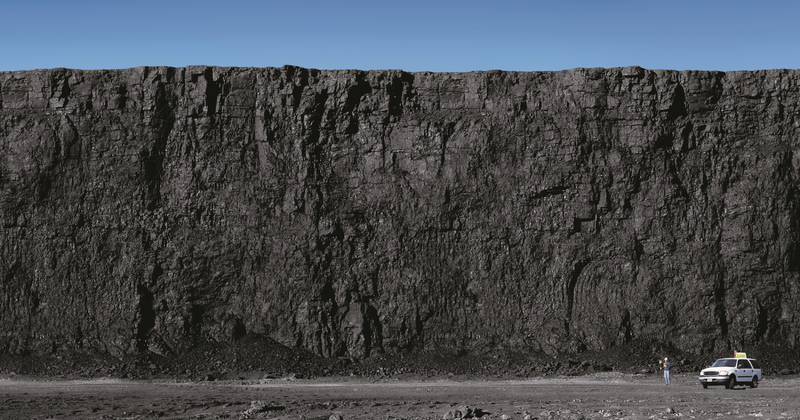 Coal seam,
  Profile of coal sulfur content.
 Yearly coal flows between different US Census Divisions.
 Yearly profiles of US electricity generation by carbon intensity.
 Percent of CO2 emissions coming from percent of electricity generation.
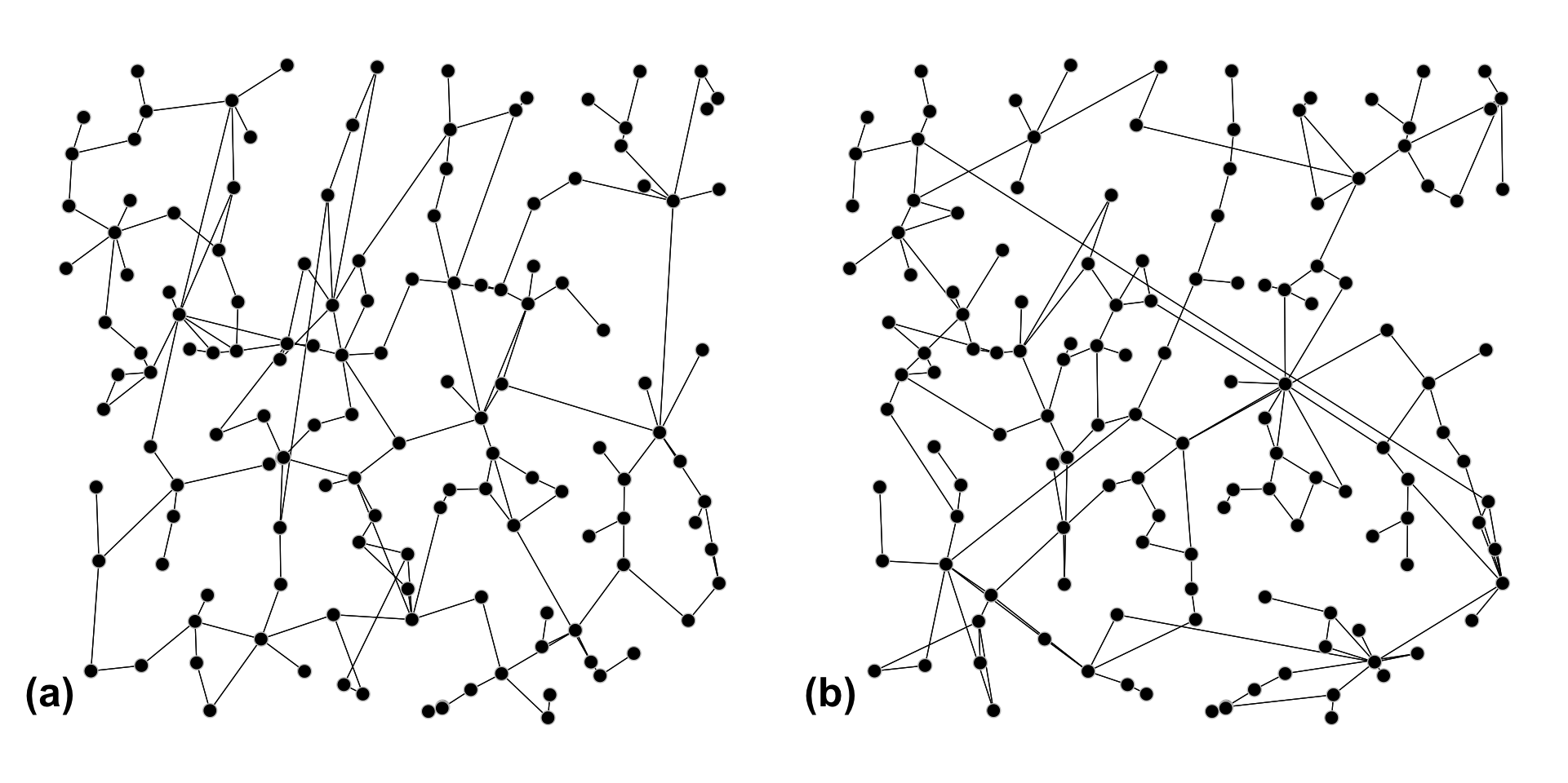 Visualisation of two grids generated using the procedure described here. Notice that both present the same bus locations, as their placement is entirely deterministic. The transmission line topology however is different in each case, as it is generated through an stochastic process. Note that the generated grids are non-planar.
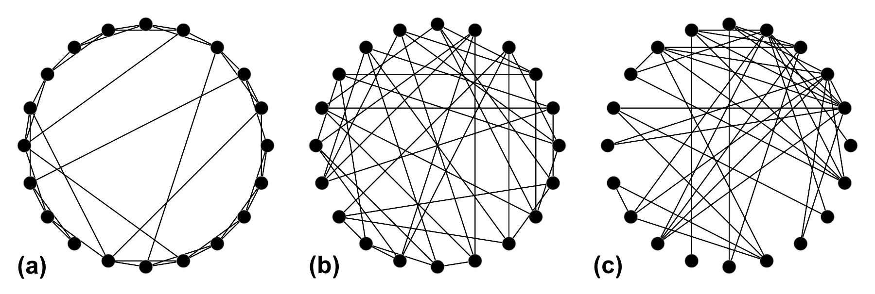 Some examples of different network topologies containing 20 nodes and 40 edges. (a) Small-world; (b) random; (c) scale-free (exponent 2). For more details, see Watts and Strogatz