The Emergent Features of JuliaLang: Part I

Author: Frames Catherine White

Introduction

This blog post is based on a talk originally given at a Cambridge PyData Meetup, and also at a London Julia Users Meetup.

Julia is known to be a very expressive language with many interesting features. It is worth considering that some features were not planned, but simply emerged from combinations of other features. This post will describe how several interesting features are implemented:

1. Unit syntactic sugar,
2. Pseudo-OO objects with public/private methods,
3. Dynamic Source Tranformation / Custom Compiler Passes (Cassette),
4. Traits.

Some of these (1 and 4) should be used when appropriate, while others (2 and 3) are rarely appropriate, but are instructive.

Part I of this post (which you are reading now) will focus on the first three. Part II of this post is about traits, which deserve there own section because they are one of the most powerful and interesting Julia features. They emerge from types, multiple dispatch, and the ability to dispatch on the types themselves (rather than just instances). We will review both the common use of traits on types, and also the very interesting—but less common—use of traits on functions.

There are many other emergent features which are not discussed in this post. For example, creating a vector using Int[] is an overload of getindex, and constructors are overloads of ::Type{<:T}().

Juxtaposition Multiplication: Convenient Syntax for Units

Using units in certain kinds of calculations can be very helpful for protecting against arithmetic mistakes. The package Unitful provides the ability to do calculations using units in a very natural way, and makes it easy to write things like “2 meters” as 2m. Here is an example of using Unitful units:

julia> using Unitful.DefaultSymbols

julia> 1m * 2m
2 m^2

julia> 10kg * 15m / 1s^2
150.0 kg m s^-2

julia> 150N == 10kg * 15m / 1s^2
true

How does this work? The answer is Juxtaposition Multiplication—a literal number placed before an expression results in multiplication:

julia> x = 0.5π
1.5707963267948966

julia> 2x
3.141592653589793

julia> 2sin(x)
2.0

To make this work, we need to overload multiplication to invoke the constructor of the unit type. Below is a simplified version of what goes on under the hood of Unitful.jl:

abstract type Unit<:Real end
struct Meter{T} <: Unit
    val::T
end

Base.:*(x::Any, U::Type{<:Unit}) = U(x)

Here we are overloading multiplication with a unit subtype, not an instance of a unit subtype (Meter(2)), but with the subtype itself (Meter). This is what ::Type{<:Unit} refers to. We can see this if we write:

julia> 5Meter
Meter{Int64}(5)

This shows that we create a Meter object with val=5.

To get to a full units system, we then need to define methods for everything that numbers need to work with, such as addition and multiplication. The final result is units-style syntactic sugar.

Closures give us “Classic Object-Oriented Programming”

First, it is important to emphasize: don’t do this in real Julia code. It is unidiomatic, and likely to hit edge-cases the compiler doesn’t optimize well (see for example the infamous closure boxing bug). This is all the more important because it often requires boxing (see below).

“Classic OO” has classes with member functions (methods) that can see all the fields and methods, but that outside the methods of the class, only public fields and methods can be seen. This idea was originally posted for Julia in one of Jeff Bezanson’s rare Stack Overflow posts, which uses a classic functional programming trick.

Let’s use closures to define a Duck type as follows:

function newDuck(name)
    # Declare fields:
    age=0

    # Declare methods:
    get_age() = age
    inc_age() = age+=1

    quack() = println("Quack!")
    speak() = quack()

    #Declare public:
    ()->(get_age, inc_age, speak, name)
end

This implements various things we would expect from “classic OO” encapsulation. We can construct an object and call public methods:

julia> bill_the_duck = newDuck("Bill")
#7 (generic function with 1 method)

julia> bill_the_duck.get_age()
0

Public methods can change private fields:

julia> bill_the_duck.inc_age()
1

julia> bill_the_duck.get_age()
1

Outside the class we can’t access private fields:

julia> bill_the_duck.age
ERROR: type ##7#12 has no field age

We also can’t access private methods:

julia> bill_the_duck.quack()
ERROR: type ##7#12 has no field quack

However, accessing their functionality via public methods works:

julia> bill_the_duck.speak()
Quack!

How does this work?

Closures return singleton objects, with directly-referenced, closed variables as fields. All the public fields/methods are directly referenced, but the private fields (e.g age, quack) are not—they are closed over other methods that use them. We can see those private methods and fields via accessing the public method closures:

julia> bill_the_duck.speak.quack
(::var"#quack#10") (generic function with 1 method)

julia> bill_the_duck.speak.quack()
Quack!

julia> bill_the_duck.inc_age.age
Core.Box(1)

An Aside on Boxing

The Box type is similar to the Ref type in function and purpose. Box is the type Julia uses for variables that are closed over, but which might be rebound to a new value. This is the case for primitives (like Int) which are rebound whenever they are incremented. It is important to be clear on the difference between mutating the contents of a variable, and rebinding that variable name.

julia> x = [1, 2, 3, 4];

julia> objectid(x)
0x79eedc509237c203

julia> x .= [10, 20, 30, 40];  # mutating contents

julia> objectid(x)
0x79eedc509237c203

julia> x = [100, 200, 300, 400];  # rebinding the variable name

julia> objectid(x)
0xfa2c022285c148ed

In closures, boxing applies only to rebinding, though the closure bug means Julia will sometimes over-eagerly box variables because it believes that they might be rebound. This has no bearing on what the code does, but it does impact performance.

While this kind of code itself should never be used (since Julia has a perfectly functional system for dispatch and works well without “Classic OO”-style encapsulation), knowing how closures work opens other opportunities to see how they can be used. In our ChainRules.jl project, we are considering the use of closures as callable named tuples as part of a difficult problem in extensibility and defaults.

Cassette, etc.

Cassette is built around a notable Julia feature, which goes by several names: Custom Compiler Passes, Contextual Dispatch, Dynamically-scoped Macros or Dynamic Source Rewriting. This same trick is used in IRTools.jl, which is at the heart of the Zygote automatic differentiation package. This is an incredibly powerful and general feature, and was the result of a very specific Issue #21146 and very casual PR #22440 suggestion that it might be useful for one particular case. These describe everything about Cassette, but only in passing.

The Custom Compiler Pass feature is essential for:

• AutoDiff tools (ForwardDiff2, Zygote, Yota),
• Mocking tools (SimpleMock.jl),
• Debuggers (MagneticReadHead, MixedModeDebugger.jl),
• Code-proof related tools (ConcolicFuzzer.jl),
• Generally rewriting all the code (GPUifyLoops.jl).

Call Overloading

One of the core uses of Cassette is the ability to effectively overload what it means to call a function. Call overloading is much more general than operator overloading, as it applies to every call (special-cased as appropriate), whereas operator overloading applies to just one function call and just one set of types.

To give a concrete example of how call overloading is more general, operator overloading/dispatch (multiple or otherwise) would allow us to to overload, for example, sin(::T) for different types T. This way sin(::DualNumber) could be specialized to be different from sin(::Float64), so that with DualNumber as input it could be set to calculate the nonreal part using the cos (which is the derivative of sin). This is exactly how DualNumbers operate. However, operator overloading can’t express the notion that, for all functions f, if the input type is DualNumber, that f should calculate the dual part using the deriviative of f. Call overloading allows for much more expressivity and massively simplifies the implementation of automatic differentiation.

The above written out in code:

function Cassette.overdub(::AutoDualCtx, f, d::DualNumber)
    res = ChainRules.frule(f, val(d))
    if res !== nothing
        f_val, pushforward = res
        f_diff = pushforward(partial(f))
        return Dual(f_val, extern(f_diff))
    else
        return f(d)
    end
end

That is just one of the more basic things that can be done with Cassette. Before we can explain how Cassette works, we need to understand how generated functions work, and before that we need to understand the different ways code is presented in Julia, as it is compiled.

Layers of Representation

Julia has many representations of the code it moves through during compilation.

• Source code (CodeTracking.definition(String,....)),
• Abstract Syntax Tree (AST): (CodeTracking.definition(Expr, ...),
• Untyped Intermediate Represention (IR): @code_lowered,
• Typed Intermediate Represention: @code_typed,
• LLVM: @code_llvm,
• ASM: @code_native.

We can retrieve the different representations using the functions/macros indicated.

The Untyped IR is of particular interest as this is what is needed for Cassette. This is a linearization of the AST, with the following properties:

• Only 1 operation per statement (nested expressions get broken up);
• the return values for each statement are accessed as SSAValue(index);
• variables become Slots;
• control-flow becomes jumps (like Goto);
• function names become qualified as GlobalRef(mod, func).

Untyped IR is stored in a CodeInfo object. It is not particularly pleasent to write, though for a intermidate representation it is fairly readable. The particularly hard part is that expression return values are SSAValues which are defined by position. So if code is added, return values need to be renumbered. Core.Compiler, Cassette and IRTools define various helpers to make this easier, but for out simple example we don’t need them.

Generated Functions

Generated functions take types as inputs and return the AST (Abstract Syntax Tree) for what code should run, based on information in the types. This is a kind of metaprogramming. Take for example a function f with input an N-dimensional array (type AbstractArray{T, N}). Then a generated function for f might construct code with N nested loops to process each element. It is then possible to generate code that only accesses the fields we want, which gives substantial performance improvements.

For a more detailed example lets consider merging NamedTuples. This could be done with a regular function:

function merge(a::NamedTuple{an}, b::NamedTuple{bn}) where {an, bn}
    names = merge_names(an, bn)
    types = merge_types(names, typeof(a), typeof(b))
    NamedTuple{names,types}(map(n->getfield(sym_in(n, bn) ? b : a, n), names))
end

This checks at runtime what fields each NamedTuple has, in order to decide what will be in the merge. However, we actually know all this information based on the types alone, because a list of fields is stored as part of the type (that is the an and bn type-parameters.)

@generated function merge(a::NamedTuple{an}, b::NamedTuple{bn}) where {an, bn}
    names = merge_names(an, bn)
    types = merge_types(names, a, b)
    vals = Any[ :(getfield($(sym_in(n, bn) ? :b : :a), $(QuoteNode(n)))) for n in names ]
    :( NamedTuple{$names,$types}(($(vals...),)) )
end

Recall that a generated function returns an AST, which is the case in the examples above. However, it is also allowed to return a CodeInfo for Untyped IR.

Making Cassette

There are two key facts mentioned above:

1. Generated Functions are allowed to return CodeInfo for Untyped IR.
2. @code_lowered f(args...) provided the ability to retrieve the CodeInfo for the given method of f.

The core of Cassete it to use a generated function to call code defined in a new CodeInfo of Untyped IR, which is based on a modified copy of code that is returned by @code_lowered. To properly understand how it works, lets run through a manual example (originally from a JuliaCon talk on MagneticReadHead.jl).

We define a generated function rewritten that makes a copy of the Untyped IR (a CodeInfo object that it gets back from @code_lowered) and then mutates it, replacing each call with a call to the function call_and_print. Finally, this returns the new CodeInfo to be run when it is called.

call_and_print(f, args...) = (println(f, " ", args); f(args...))


@generated function rewritten(f)
    ci_orig = @code_lowered f.instance()
    ci = ccall(:jl_copy_code_info, Ref{Core.CodeInfo}, (Any,), ci_orig)
    for ii in eachindex(ci.code)
        if ci.code[ii] isa Expr && ci.code[ii].head==:call
            func = GlobalRef(Main, :call_and_print)
            ci.code[ii] = Expr(:call, func, ci.code[ii].args...)
        end
    end
    return ci
end

(Notice: this exact version of the code works on julia 1.0, 1.1, and 1.2, and also prints a ton of warnings as it hurts type-inference a lot. But slightly improved versions of it exist in Cassette, that don’t make type-inference cry, and that work in all Julia versions. This just gets the point across.)

We can see that this works:

julia> foo() = 2*(1+1)
foo (generic function with 1 method)

julia> rewritten(foo)
+ (1, 1)
* (2, 2)
4

Rather than replacing each call with call_and_print, we could instead call a function that does the work we are interested in, and then calls rewritten on the function that would have been called:

function work_and_recurse(f, args...)
    println(f, " ", args)
    rewritten(f, args...)
end

So, not only does the function we call get rewritten, but so does every function it calls, all the way down.

This is how Cassette and IRTools work. There are a few complexities and special cases that need to be taken care of, but this is the core of it: recursive invocation of generated functions that rewrite the IR, similar to what is returned by @code_lowered.

Wrapping up Part I

In this part we covered the basics of:

1. Unit syntactic sugar,
2. Pseudo-OO objects with public/private methods,
3. Dynamic Source Tranformation / Custom Compiler Passes (Cassette).

In Part II, we will discuss Traits!

Memristive dynamics: a heuristic optimization tool

Author: Ana Zegarac and Francesco Caravelli

\(\newcommand{\Ron}{R_{\text{on}}}\) \(\newcommand{\Roff}{R_{\text{off}}}\) \(\newcommand{\dif}{\mathop{}\!\mathrm{d}}\) \(\newcommand{\coloneqq}{\mathrel{\vcenter{:}}=}\)

Introduction

In this post we will explore an interesting area of modern circuit theory and computing: how exotic properties of certain nanoscale circuit components (analogous to tungsten filament lightblulbs) can be used for solving certain optimization problems. Let’s start with a simple example: imagine a circuit made up of resistors, all of which have the same resistance.

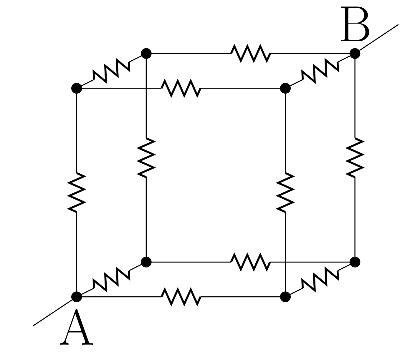
If we connect points A and B of the circuit above to a battery, current will flow through the conductors (let’s say from A to B), according to Kirchhoff’s laws. Because of the symmetry of the problem, the current splits at each intersection according to the inverse resistance rule, and so the currents will flow equally in all directions to reach B. This implies that if we follow the maximal current at each intersection, we can use this circuit to solve the minimum distance (or cost) problem on a graph. This can be seen as an example of a physical system performing analog computation. More generally, there is a deep connection between graph theory and resistor networks.

In 2008, researchers from Hewlett Packard introduced what is now called the “nanoscale memristor” ¹. This is a type of resistor made of certain metal oxides such as tungsten or titanium, for which the resistance changes as a function of time in a peculiar way. For the case of titanium dioxide, the resistance changes between two limiting values according to a simple convex law depending on an internal parameter, \(w\), which is constrained between \(0\) and \(1\):

where,

and \(I\) is the current in the device. This is a simple prototypical model of a memory-resistor, or memristor.

In the general case of a network of memristors, the above differential equation becomes ^{2 3 4 5}:

where \(\Omega\) is a matrix representing the circuit topology, \(\vec S(t)\) are the applied voltages, and \(W\) a diagonal matrix of the values of \(w\) for each memristor in the network.

It is interesting to note that the equation above is related to a class of optimization problems, similarly to the case of a circuit of simple resistors. In the memristor case, this class is called quadratically unconstrained binary optimization (QUBO). The solution of a QUBO problem is the set of binary parameters, \(w_i\), that minimize (or maximize) a function of the form:

This is because the dynamics of memristors, which are described by the equation above, is such that a QUBO functional is minimized. For the case of realistic circuits, \(\Omega\) satisfies certain properties which we will discuss below, but from the point of view of optimization theory, the system of differential equations can in principle be simulated for arbitrary \(\Omega\). Therefore, the memristive differential equation can serve as a heuristic solution method for an NP-Complete problem such as QUBO ⁴. These problems are NP-Complete because there is no known algorithm that is better than exhaustive search: because of the binary nature of the variables, in the worst case we have to explore all \(2^N\) possible values of the variables \(w\) to find the extrema of the problem. In a sense, the memristive differential equation is a relaxation of the QUBO problem to continuous variables.

Let’s look at an application to a standard problem: given the expected returns and covariance matrix between prices of some financial assets, which assets should an investor allocate capital to? This setup, with binary decision variables, is different than the typical question of portfolio allocation, in which the decision variables are real valued (fractions of wealth to allocate to assets). This is a combinatorial decision whether or not to invest in a given asset, but not the amount: the combinatorial Markowitz problem. The heuristic solution we propose has been introduced in the appendix of this paper. This can also be used as a screening procedure before the real portfolio optimization is performed, i.e., as a dimensionality reduction technique. More formally, the objective is to maximize:

where \(r_i\) are the expected returns and \(\Sigma\) the covariance matrix. The mapping between the above and the equivalent memristive equation is given by:

The solution vector \(S\) is obtained through inversion of the matrix \(\Sigma\) (if it is invertible). There are some conditions for this method to be suitable for heuristic optimization (related to the spectral properties of the matrix \(J\)), but as a heuristic method, this is much cheaper than exhaustive search: it requires a single matrix inversion which scales as \(O(N^3)\), and the simulation of a first order differential equation which also requires a matrix inversion step by step, and thus scales as \(O(T \cdot N^3)\) where \(T\) is the number of time steps. We propose two approaches to this problem: one based on the most common Metropolis-Hasting-type algorithm (at each time step we flip a single weight, which can be referred as “Gibbs sampling”), and the other on the heuristic memristive equation.

Sample implementation

Below we include julia code for both algorithms.

using FillArrays
using LinearAlgebra

"""
    monte_carlo(
        expected_returns::Vector{Float64},
        Σ::Matrix{Float64},
        p::Float64,
        weights_init::Vector{Bool};
        λ::Float64=0.999995,
        effective_its::Int=3000,
        τ::Real=0.75,
    )

Execute Monte Carlo in order to find the optimal portfolio composition,
considering an asset covariance matrix `Σ` and a risk parameter `p`. `reg`
represents the regularisation constant for `Σ`, `λ` is the annealing factor, with
the temperature `τ` decreases at each step and `effective_its` determines how
many times, on average, each asset will have its weight changed.
"""
function monte_carlo(
    expected_returns::Vector{Float64},
    Σ::Matrix{Float64},
    p::Float64,
    weights_init::Vector{Bool};
    λ::Float64=0.999995,
    effective_its::Int=3000,
    τ::Real=0.75,
)
    weights = weights_init
    n = size(weights_init, 1)

    total_time = effective_its * n
    energies = Vector{Float64}(undef, total_time)

    # Compute energy of initial configuration
    energy_min = energy(expected_returns, Σ, p, weights_init)

    for t in 1:total_time
        # Anneal temperature
        τ = τ * λ
        # Randomly draw asset
        rand_index = rand(1:n)
        weights_current = weights
        # Flip weight from 0 to 1 and vice-versa
        weights_current[rand_index] = 1 - weights_current[rand_index]
        # Compute new energy
        energy_current = energy(expected_returns, Σ, p, weights)

        # Compute Boltzmann factor
        β = exp(-(energy_current - energy_min) / τ)

        # Randomly accept update
        if rand() < min(1, β)
            energy_min = energy_current
            weights = weights_current
        end

        # Store current best energy
        energies[t] = energy_min
    end
    return weights, energies
end

"""
    memristive_opt(
        expected_returns::Vector{Float64},
        Σ::Matrix{Float64},
        p::Float64,
        weights_init::Vector{<:Real};
        α=0.1,
        β=10,
        δt=0.1,
        total_time=3000,
    )

Execute optimisation via the heuristic "memristive" equation in order to find the
optimal portfolio composition, considering an asset covariance matrix `Σ` and a
risk parameter `p`. `reg` represents the regularisation constant for `Σ`, `α` and
`β` parametrise the memristor state (see Equation (2)),
`δt` is the size of the time step for the dynamical updates and `total_time` is
the number of time steps for which the dynamics will be run.
"""
function memristive_opt(
    expected_returns::Vector{Float64},
    Σ::Matrix{Float64},
    p::Float64,
    weights_init::Vector{<:Real};
    α=0.1,
    β=10,
    δt=0.1,
    total_time=3000,
)
    n = size(weights_init, 1)

    weights_series = Matrix{Float64}(undef, n, total_time)
    weights_series[:, 1] = weights_init
    energies = Vector{Float64}(undef, total_time)
    energies[1] = energy(expected_returns, Σ, p, weights_series[:, 1])

    # Compute resistance change ratio
    ξ = p / 2α
    # Compute Σ times applied voltages matrix
    ΣS = β * (α/2 * ones(n, 1) + (p/2 + α * ξ/3) * diag(Σ) - expected_returns)

    for t in 1:total_time-1
        update = δt * (α * weights_series[:, t] - 1/β * (Eye(n) + ξ *
            Σ * Diagonal(weights_series[:, t])) \ ΣS)
        weights_series[:, t+1] = weights_series[:, t] + update

        weights_series[weights_series[:, t+1] .> 1, t+1] .= 1.0
        weights_series[weights_series[:, t+1] .< 1, t+1] .= 0.0

        energies[t + 1] = energy(expected_returns, Σ, p, weights_series[:, t+1])
    end

    weights_final = weights_series[:, end]

    return weights_final, energies
end

"""
    energy(
        expected_returns::Vector{Float64},
        Σ::Matrix{Float64},
        p::Float64,
        weights::Vector{Float64},
    )

Return minus the expected return corrected by the variance of the portfolio,
according to the Markowitz approach. `Σ` represents the covariance of the assets,
`p` controls the risk tolerance and `weights` represent the (here binary)
portfolio composition.
"""
function energy(
    expected_returns::Vector{Float64},
    Σ::Matrix{Float64},
    p::Float64,
    weights::Vector{<:Real},
)
    -dot(expected_returns, weights) + p/2 * weights' * Σ * weights
end

A simple comparison between the two approaches shows the superiority of the memristor equation-based approach for this problem. We used a portfolio of 200 assets, with randomly generated initial allocations, expected returns and covariances. After 3000 effective iterations (that is 3000 times 200, the number of assets), the Monte Carlo approach leads to a corrected expected portfolio return of 3.9, while the memristive approach, in only a few steps, already converges to a solution with a corrected expected portfolio return of 19.5! Moreover, the solution found via Monte Carlo allocated investment to 91 different assets, while the memristor-based one only invested in 71 assets, thus showing an even better return to investment. There are obvious caveats here, as each of these methods have their own parameters which can be tuned in order to improve performance (which we did try doing), and it is known that Monte Carlo methods are ill-suited to combinatorial problems. Yet, such a stark difference shows how powerful memristors can be for optimization purposes (in particular for quickly generating some sufficiently good but not necessarily optimal solutions).

The equation for memristors is also interesting in other ways, for example, it has graph theoretical underpinnings ^{2 3 4}. Further, the memristor network equation is connected to optimization ^{5 6 7}. These are summarized in ⁸. For a general overview of the field of memristors, see the recent review ⁹.

JuliaCon 2019

Author: Eric Davies, Fernando Chorney, Glenn Moynihan, Frames Catherine White, Mary Jo Ramos, Nicole Epp, Sean Lovett, Will Tebbutt

Some of us at Invenia recently attended JuliaCon 2019, which was held at the University of Maryland, Baltimore, on July 21-26.

It was the biggest JuliaCon yet, with more than 370 participants, but still had a welcoming atmosphere as in previous years. There were plenty of opportunities to catch up with people that you work with regularly but almost never actually have a face-to-face conversation with.

We sent 16 developers and researchers from our Winnipeg and Cambridge offices. As far as we know, this was the largest contingent of attendees after Julia Computing! We had a lot of fun and thought it would be nice to share some of our favourite parts.

Julia is more than scientific computing

For someone who is relatively new to Julia, it may be difficult to know what to expect from a JuliaCon. Consider someone who has used Julia before in a few ways, but who has yet to fully grasp the power of the language.

One of the first things to notice is just how diverse the language is. It may initially seem as a very special tool for the scientific community, but the more one learns about it, the more evident it becomes that it could be used to tackle all sorts of problems.

Workshops were tailored for individuals with a range of Julia knowledge. Beginners had the opportunity to play around with Julia in basic workshops, and more advanced workshops covered topics from differential equations to parallel computing. There was something for everyone and no reason to feel intimidated.

The Intermediate Julia for Scientific Computing workshop highlighted Julia’s multiple dispatch and meta-programming capabilities. Both are very useful and interesting tools. As one learns more about Julia and sees the growth of the community, it becomes easier to understand the reasons why some love the language so much. It has the scientific usage without compromising on speed, readability, or usefulness.

Julia is welcoming!

The various workshops and talks that encouraged diverse groups to utilize and contribute to the language were also great to see. It is uplifting to witness such a strong initiative to make everyone feel welcome.

The Diversity and Inclusion BOF provided a space for anyone to voice opinions, concerns and suggestions on how to improve the Julia experience for everyone. The Diversity and Inclusion session showcased how to foster the community’s growth. The speakers were educators who shared their experiences using Julia as a tool to enhance education for women, minorities, and students with lower socioeconomic backgrounds. The inspirational work done by these individuals – and everyone at JuliaCon – prove that anyone can use Julia and succeed with the community’s support.

The community has a big role to play

Heather Miller’s keynote on Scala’s experience as an open source project was another highlight. It is staggering to see what the adoption of open source software in industry looks like, as well as learning about the issues that come up with growth, and the importance of the community. Although Heather’s snap polls at the end seemed broadly positive about the state of Julia’s community, they suggested that the level to which we’re mentoring newer members of the community is lower than ideal.

Birds of a Feather Sessions

This year Birds of a Feather (BoF) sessions were a big thing. In previous JuliaCons, there were only one or two, but this year we had twelve. Each session was unique and interesting, and in almost every case people wished they could continue after the hour was up. The BoFs were an excellent chance to discuss and explore topics that are difficult to do in a formal talk. In many ways this is the best reason to go to a conference: to connect with people, make plans, and learn deeply. Normally this happens in cramped corridors or during coffee breaks, which certainly did happen this year still, but the BoFs gave the whole process just a little bit more structure, and also tables.

Each BoF was different and good in its own ways, and none would have been half as good without getting everyone in the same room. We mentioned the Diversity BoF earlier. The Parallelism BoF ended with everyone breaking into four groups, each of which produced notes on future directions for parallelism in Julia. Our own head of development, Curtis Vogt, ran the “Julia In Production” BoF which showed that both new and established companies are adopting Julia, and led to some useful discussion about better support for Julia in Cloud computing environments.

The Cassette BoF was particularly good. It had everyone talking about what they were using Cassette for. Our own Frames Catherine White presented his new Cassette-like project, Arborist, and some of the challenges it faces, including understanding of why the compiler behaves the way it does. We also learned that neither Jarret Revels (the creator of Cassette), nor Valentin Churavy (its current maintainer) know exactly what Tagging in Cassette does.

Support tools are becoming well established

With the advent of Julia 1.0 at JuliaCon 2018 we saw the release of a new Pkg.jl; a far more robust and user-friendly package manager. However, many core tools to support the maturing package ecosystem were yet to emerge until JuliaCon 2019. This year we saw the introduction of a new debugger, a formatter, and an impressive documentation generator.

For the past year, the absence of a debugger that equalled the pleasure of using Pkg.jl remained an open question. An answer was unveiled in Debugger.jl, by the venerable Tim Holy, Sebastian Pfitzner, and Kristoffer Carlsson. They discussed the ease with which Debugger.jl can be used to declare break points, enter functions, traverse lines of code, and modify environment variables, all from within a new debugger REPL mode! This is a very welcome addition to the Julia toolbox.

Style guides are easy to understand but it’s all too easy to misstep in writing code. Dominique Luna gave a simple walkthrough of his JuliaFormatter.jl package, which formats the line width of source code according to specified parameters. The formatter spruces up and nests lines of code to present more aesthetically pleasing text. Only recently registered as a package, and not a comprehensive linter, it is still a good step in the right direction, and one that will save countless hours of code review for such a simple package.

Code is only as useful as its documentation and Documenter.jl is the canonical tool for generating package documentation. Morten Piibeleht gave an excellent overview of the API including docstring generation, example code evaluation, and using custom CSS for online manuals. A great feature is the inclusion of doc testing as part of a unit testing set up to ensure that examples match function outputs. While Documenter has had doctests for a long time, they are now much easier to trigger: just add using Documenter, MyPackage; doctest(MyPackage) to your runtests.jl file. Coupled with Invenia’s own PkgTemplates.jl, creating a maintainable package framework has never been easier.

Probabilistic Programming: Julia sure does do a lot of it

Another highlight was the somewhat unexpected probabilistic programming track on Thursday afternoon. There were 5 presentations, each on a different framework and take on what probabilistic programming in Julia can look like. These included a talk on Stheno.jl from our own Will Tebbutt, which also contained a great introduction to Gaussian Processes.

Particularly interesting was the Gen for data cleaning talk by Alex Law. This puts the problem of data cleaning – correcting miss-entered, or incomplete data – into a probabilistic programming setting. Normally this is done via deterministic heuristics, for example by correcting spelling by using the Damerau–Levenshtein distance to the nearest word in a dictionary. However, such approaches can have issues, for instance, when correcting town names, the nearest by spelling may be a tiny town with very small population, which is probably wrong. More complicated heuristics can be written to handle such cases, but they can quickly become unwieldy. An alternative to heuristics is to write statements about the data in a probabilistic programming language. For example, there is a chance of one typo, and a smaller chance of two typos, and further that towns with higher population are more likely to occur. Inference can then be run in the probabilistic model for the most likely cleaned field values. This is a neat idea based on a few recent publications. We’re very excited about all of this work, and look forward to further discussions with the authors of the various frameworks.

Composable Parallelism

A particularly exciting announcement was composable multi-threaded parallelism for Julia v1.3.0-alpha.

Safe and efficient thread parallelism has been on the horizon for a while now. Previously, multi-thread parallelism was in an experimental form and generally very limited (see the Base.Threads.@threads macro). This involved dividing the work into blocks that execute independently and then joined into Julia’s main thread. Limitations included not being able to use I/O or to do task switching inside the threaded for-loop of parallel work.

All that is changing in Julia v1.3. One of the most exciting changes is that all system-level I/O operations are now thread-safe. Functions like print can be used during a @spawn or @threads macro for-loop call. Additionally, the @spawn construct (which is like @async, but parallel) was introduced; this has a threaded meaning, moving towards parallelism rather than the pre-existing Distributed standard library export.

Taking advantage of hardware parallel computing capacities can lead to very large speedups for certain workflows, and now it will be much easier to get started with threads. The usual multithreading pitfalls of race conditions and potential deadlocks still exist, but these can generally be worked around with locks and atomic operations where needed. There are many other features and improvements to look forward to.

Neural differential equations: machine learning and physics join forces

We were excited to see DiffEqFlux.jl presented at JuliaCon this year. This combines the excellent DifferentialEquations.jl and Flux.jl packages to implement Neural ODEs, SDEs, PDEs, DDEs, etc. All using state-of-the-art time-integration methods.

The Neural Ordinary Differential Equations paper caused a stir at NeurIPS 2018 for its successful combination of two seemingly-distinct techniques: differential equations and neural networks. More generally there has been a recent resurgence of interest in combining modern machine learning with traditional scientific modelling techniques (see Hidden Physics Models, among others). There are many possible applications for these methods: they have potential for both enriching black-box machine learning models with physical insights, and conversely using data to learn unknown terms in structured physical models. For example, it is possible to use a differential equations solver as a layer embedded within a neural network, and train the resulting model end-to-end. In the latter case, it is possible to replace a term in a differential equation by a neural network. Both these use-cases, and many others, are now possible in DiffEqFlux.jl with just a few lines of code. The generic programming capabilities of Julia really shine through in the flexibility and composability of these tools, and we’re excited to see where this field will go next.

The compiler has come a long way!

The Julia compiler and standard library has come a long way in the last two years. An interesting case came up while Eric Davies was working on IndexedDims.jl at the hackathon.

Take for example the highly-optimized code from base/multidimensional.jl: ​

@generated function _unsafe_getindex!(dest::AbstractArray, src::AbstractArray, I::Vararg{Union{Real, AbstractArray}, N}) where N
   quote
       Base.@_inline_meta
       D = eachindex(dest)
       Dy = iterate(D)
       @inbounds Base.Cartesian.@nloops $N j d->I[d] begin
           # This condition is never hit, but at the moment
           # the optimizer is not clever enough to split the union without it
           Dy === nothing && return dest
           (idx, state) = Dy
           dest[idx] = Base.Cartesian.@ncall $N getindex src j
           Dy = iterate(D, state)
       end
       return dest
   end
end

It is interesting that this now has speed within a factor of two of the following simplified version:

function _unsafe_getindex_modern!(dest::AbstractArray, src::AbstractArray, I::Vararg{Union{Real, AbstractArray}, N}) where N
   @inbounds for (i, j) in zip(eachindex(dest), Iterators.product(I...))
       dest[i] = src[j...]
   end
   return dest
end

In Julia 0.6, this was five times slower than the highly-optimized version above!

It turns out that the type parameter N matters a lot. Removing this explicit type parameter causes performance to degrade by an order of magnitude. While Julia generally specializes on the types of the arguments passed to a method, there are a few cases in which Julia will avoid that specialization unless an explicit type parameter is added: the three main cases are Function, Type, and as in the example above, Vararg arguments.

Some of our other favourite talks

Here are some of our other favourite talks not discussed above:

1. Heterogeneous Agent DSGE Models
2. Solving Cryptic Crosswords
3. Differentiate All The Things!
4. Building a Debugger with Cassette
5. FilePaths
6. Ultimate Datetime
7. Smart House with JuliaBerry
8. Why writing C interfaces in Julia is so easy
9. Open Source Power System Modeling
10. What’s Bad About Julia
11. The Unreasonable Effectiveness of Multiple Dispatch

It is always impressive how much is covered every JuliaCon, considering its size. It serves to show both how fast the community is growing and how versatile the language is. We look forward for another one in 2020, even bigger and broader.

Factor the Joint! Intoducing GPAR: a Multi-output GP Model

Author: James Requeima

Introduction

Gaussian processes (GP) provide a powerful and popular approach to nonlinear single-output regression. Most regression problems, however, involve multiple outputs rather than a single one. When modelling such data, it is key to capture the dependencies between the outputs. For example, noise in the output space might be correlated, or, while one output might depend on the inputs in a complex (deterministic) way, it may depend quite simply on other output variables. In such cases a multi-output model is required. Let’s examine such an example.

A Multi-output Modelling Example

Consider the problem of modelling the world’s average CO2 level \(C(t)\), temperature \(T(t)\), and Arctic sea ice extent \(I(t)\) as a function of time \(t\). By the greenhouse effect, one can imagine that the temperature \(T(t)\) is a complicated stochastic function \(f_1\) of CO2 and time: \(T(t) = f_1(C(t),t)\). Similarly, the Arctic sea ice extent \(I(t)\) can be modelled as another complicated function \(f_2\) of temperature, CO2, and time: \(I(t) = f_2(T(t),C(t),t)\). These functional relationships are depicted in the figure below:

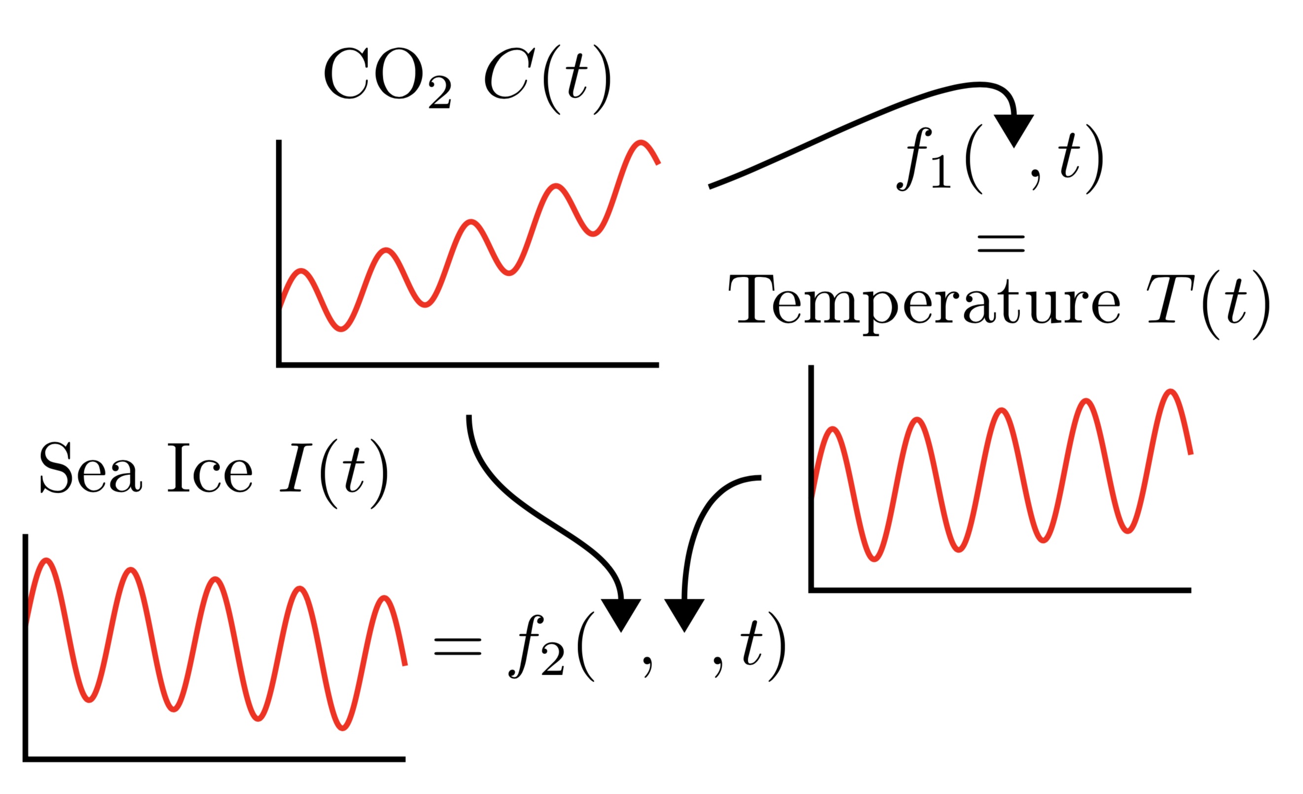
This structure motivates the following model where we have conditional probabilities modelling the underlying functions \(f_1\) and \(f_2\), and the full joint ditribution can be expressed as

More generally, consider the problem of modelling \(M\) outputs \(y_{1:M} (x) = (y1(x), . . . , yM (x))\) as a function of the input \(x\). Applying the product rule yields

which states that \(y_1(x)\), like CO2, is first generated from \(x\) according to some unknown random function \(f_1\); that \(y_2(x)\), like temperature, is then generated from \(y_1(x)\) and \(x\) according to some unknown random function \(f_2\); that \(y_3(x)\), like the Arctic sea ice extent, is then generated from \(y_2(x)\), \(y_1(x)\), and \(x\) according to some unknown random function \(f_3\); et cetera:

\begin{align} y_1(x) &= f_1(x), & f_1 &\sim p(f_1), \newline y_2(x) &= f_2(y_1(x), x), & f_2 &\sim p(f_2), \newline y_3(x) &= f_3(y_{1:2}(x), x), & f_3 &\sim p(f_3), \newline &\;\vdots \nonumber \newline y_M(x) &= f_M(y_{1:M-1}(x),x) & f_M & \sim p(f_M). \end{align}

GPAR, the Gaussian Process Autoregressive Regression Model, models these unknown functions \(f_{1:M}\) with Gaussian Processes.

Modelling According to the Product Rule

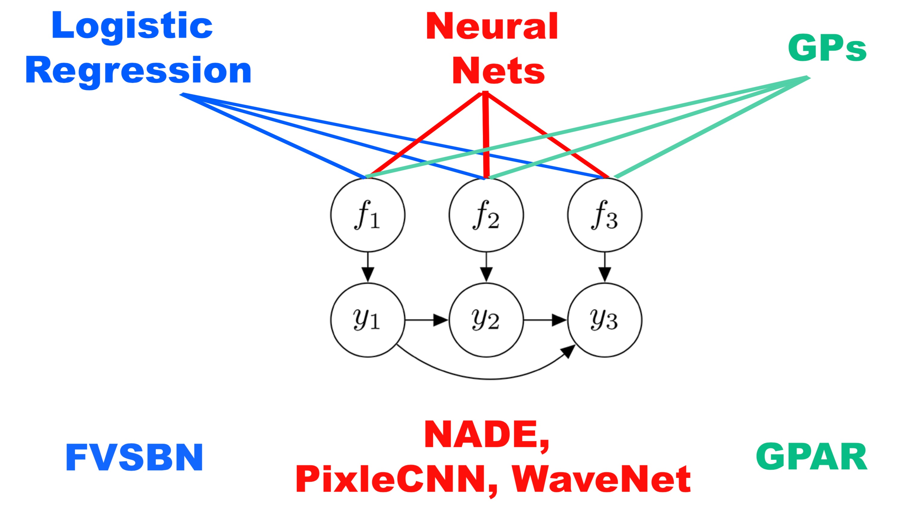
GPAR is not the first model to use the technique of factoring the joint distribution using the product rule and modelling each of the conditionals. A recognized advantage of this procedure is that if each of the individual conditional models is tractable then the entire model is also tractable. It also transforms the multi-output regression task into several single-output regression tasks which are easy to handle.

There are many interesting approaches to this problem, using various incarnations of neural networks. Neal [1992] and Frey et al. [1996] use logistic-regression-style models for the Fully Visible Sigmoid Belief Network (FVSBN), Larochelle and Murray [2011] use feed forward neural networks in NADE, and RNNs and convolutions are used in Wavenet (van den Oord et al., [2016]) and PixelCNN (van den Oord et al., [2016]).

In particular, if the observations are real-valued, a standard architecture lets the conditionals be Gaussian with means encoded by neural networks and fixed variances. Under broad conditions, if these neural networks are replaced by Bayesian neural networks with independent Gaussian priors over the weights, we recover GPAR as the width of the hidden layers goes to infinity (Neal, [1996]; Matthews et al., [2018]).

Other Multi-output GP Models

There are also many other multi-output GP models, many – but not all – of which consist of a “mixing” generative procedure: a number of latent GPs are drawn from GP priors and then “mixed” using a matrix multiplication, transforming the functions to the output space. Many of the GP based multi-output models are recoverable by GPAR, often in a much more tractable way. We discuss this further in our paper.

Some Issues With GPAR

Output Ordering

To construct GPAR, an ordering of outputs must be determined. We found that in many cases the ordering and the dependency structure of the outputs is obvious. If the order is not obvious, however, how can we choose one? We would like the ordering which maximizes the joint marginal likelihood of the entire GPAR model but, in most cases, building GPAR for all permutations of orderings is intractable. A more realistic approach would be to perform a greedy search: the first dimension would be determined by constructing a single output GP for each of the output dimensions and selecting the dimension that yields the largest marginal likelihood. The second dimension would then be selected by building a GP(AR) conditional on the first dimension and selecting the largest marginal likelihood, etc. In simple synthetic experiments, by permuting the generative ordering of observations, GPAR is able to recover the true ordering.

Missing Datapoints

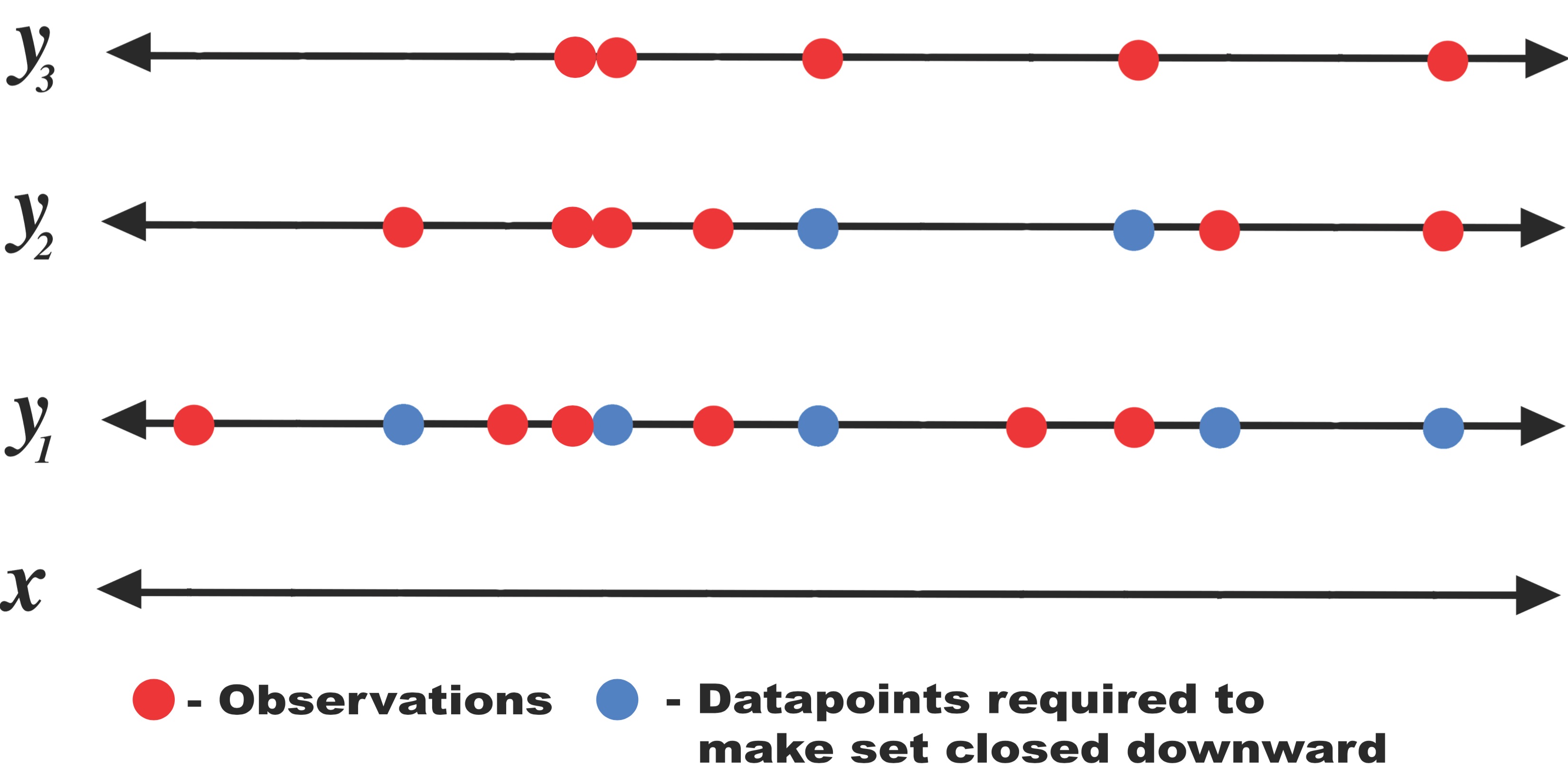
In order to use GPAR, the training dataset should be what we define to be “closed downward”: let \(D\) be a collection of observations of the form \((x, y_i)\) where \(y_i\) is observation in output dimension \(i\) at input location \(x\). \(D\) is closed downward if \((x, y_i) \in D\) implies that \((x, y_j) \in D\) for all \(j \leq i\).

This is not an issue if the dataset is complete, i.e., we have all output observations for each datapoint. However, in real-world cases some of the observations may be missing, resulting in datasets that are not closed downwards. In such cases, only certain orderings are allowed, or some parts of the dataset must be removed to construct one that is closed downwards. This could result in either a suboptimal model or in throwing away valuable information. To get around this issue, in our experiments we imputed missing values using the mean predicted by the previous conditional GP. The correct thing to do would be to sample from the previous conditional GP to integrate out the missing values, but in our experiments we found that simply using the mean works well.

What Can GPAR Do?

GPAR is well suited for problems where there is a strong functional relationship between outputs and for problems where observation noise is richly structured and input-dependent. To demonstrate this we tested GPAR on some synthetic problems.

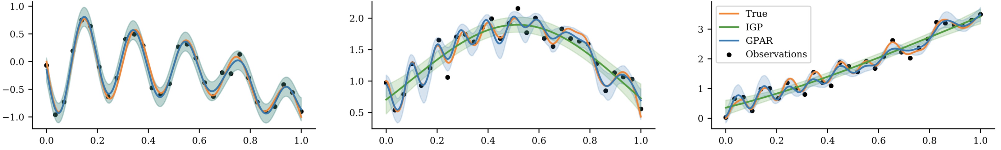
First, we test the ability to leverage strong functional relationships between the outputs. Consider three outputs \(y_1\), \(y_2\), and \(y_3\), which depend nonlinearly on each other:

\begin{align} y_1(x) &= -\sin(10\pi(x+1))/(2x + 1) - x^4 + \epsilon_1, \newline y_2(x) &= \cos^2(y_1(x)) + \sin(3x) + \epsilon_2, \newline y_3(x) &= y_2(x)y_1^2(x) + 3x + \epsilon_3, \end{align}

where \(\epsilon_1, \epsilon_2, \epsilon_3 {\sim} \mathcal{N}(0, 1)\). By substituting \(y_1\) and \(y_2\) into \(y_3\), we see that \(y_3\) can be expressed directly in terms of \(x\), but via a very complex function. This function of \(x\) is difficult to model with few data points. The dependence of \(y_3\) on \(y_1\) and \(y_2\) is much simpler. Therefore, as GPAR can exploit direct dependencies between \(y_{1:2}\) and \(y_3\), it should be presented with a simpler task compared to predicting \(y_3\) from \(x\) directly.

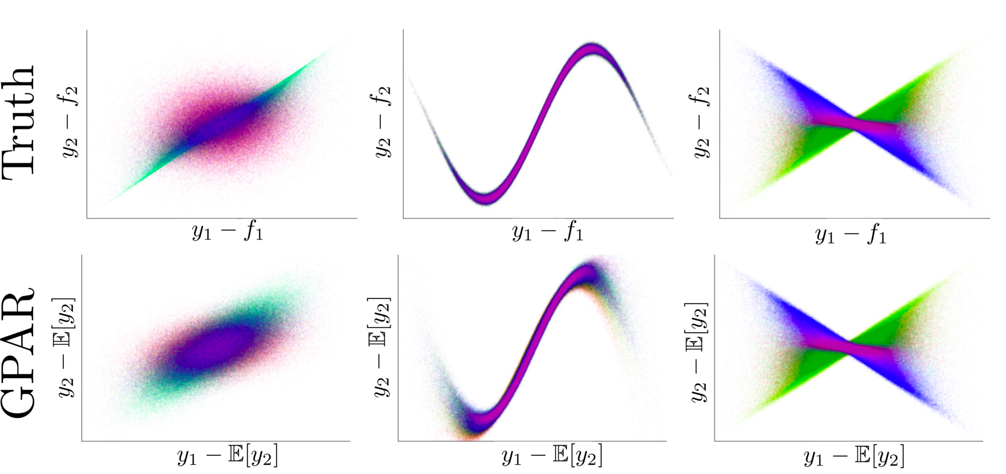
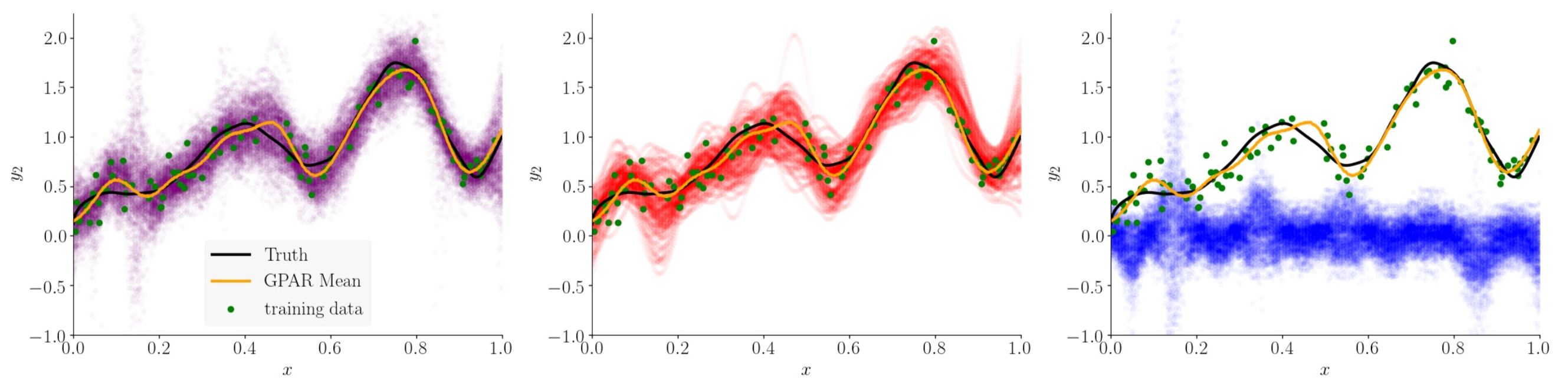
Second, we test GPAR’s ability to capture non-Gaussian and input-dependent noise. Consider the following three schemes in which two outputs are observed under various noise conditions: \(y_1(x) = f_1(x) + \epsilon_1\) and

\begin{align} \text{(1): } y_2(x) &= f_2(x) + \sin^2(2 \pi x)\epsilon_1 + \cos^2(2 \pi x) \epsilon_2, \newline \text{(2): } y_2(x) &= f_2(x) + \sin(\pi\epsilon_1) + \epsilon_2, \newline \text{(3): } y_2(x) &= f_2(x) + \sin(\pi x) \epsilon_1 + \epsilon_2, \end{align}

where \(\epsilon_1, \epsilon_2 \sim \mathcal{N}(0, 1)\), and \(f_1\) and \(f_2\) are nonlinear functions of \(x\):

\begin{align} f_1(x) &= -\sin(10\pi(x+1))/(2x + 1) - x^4 \newline f_2(x) &= \frac15 e^{2x}\left(\theta_{1}\cos(\theta_{2} \pi x) + \theta_{3}\cos(\theta_{4} \pi x) \right) + \sqrt{2x}, \end{align}

where the \(\theta\)s are constant values. All three schemes have i.i.d. homoscedastic Gaussian noise in \(y_1\) making \(y_1\) easy to learn for GPAR. The noise in \(y_2\) depends on that in \(y_1\), and can be heteroscedastic. The task for GPAR is to learn the scheme’s noise structure.

Note that we don’t have to make any spectial modelling assumptions to capture these noise structures: we still model the conditional distributions with GPs assuming i.i.d. Gaussian noise. We can now add components to our kernel composition to specifically model the structured noise. A figure below shows this decomposition.

Using the kernel decomposition it is possible to analyse both the functional and noise structure in an automated way similar to the work done by Duvenaud et al. in (Structure discovery in nonparametric regression through compositional kernel search, 2014).

Real World Benchmarks

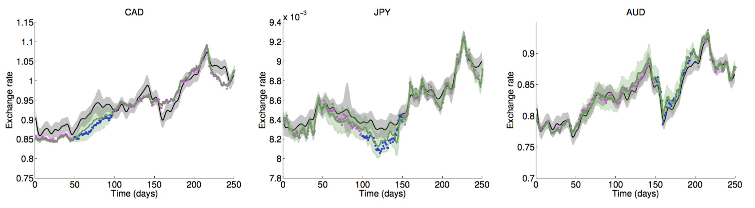
We compared GPAR to the state-of-the-art multi-output GP models on some standard benchmarks and showed that not only is GPAR often easier to implement and is faster than these methods, but it also yields better results. We tested GPAR on an EEG data set which consists of 256 voltage measurements from 7 electrodes placed on a subject’s scalp while the subject is shown a certain image; the Jura data set which comprises metal concentration measurements collected from the topsoil in a 14.5 square kilometer region of the Swiss Jura; and an exchange rates data set which consists of the daily exchange rate w.r.t. USD of the top ten international currencies (CAD, EUR, JPY, GBP, CHF,AUD, HKD, NZD, KRW, and MXN) and three preciousmetals (gold, silver, and platinum) in the year 2007. The plot below shows the comparison between GPAR and independent GPs:

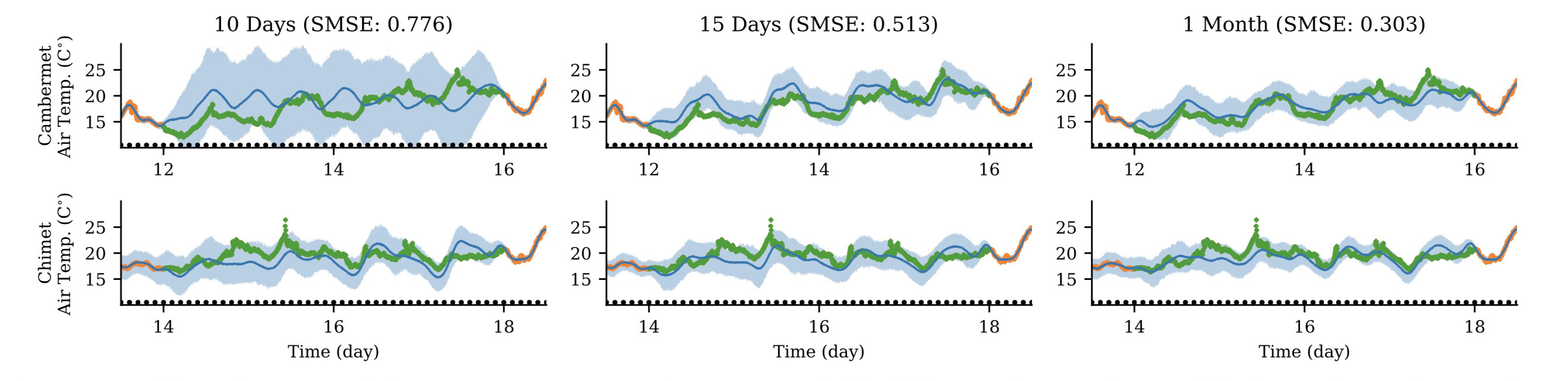
Lastly, a tidal height, wind speed, and air temperature data set (http://www.bramblemet.co.uk, http://cambermet.co.uk, http://www.chimet.co.uk, and http://sotonmet.co.uk) which was collected at 5 minute intervals by four weather stations: Bramblemet, Cambermet, Chimet, and Sotonmet, all located in Southampton, UK. The task in this last experiment is to predict the air temperature measured by Cambermet and Chimet from all other signals. Performance is measured with the SMSE. This experiment serves two purposes. First, it demonstrates that it is simple to scale GPAR to large datasets using off-the-shelf inducing point techniques for single-output GP regression. In our case, we used the variational inducing point method by Titsias (2009) with 10 inducing points per day. Second, it shows that scaling to large data sets enables GPAR to better learn dependencies between outputs, which, importantly, can significantly improve predictions in regions where outputs are partially observed. Using as training data 10 days (days [10,20), roughly 30k points), 15 days (days [18,23), roughly 47k points), and the whole of July (roughly 98k points), make predictions of 4 day periods of the air temperature measured by Cambermet and Chimet. Despite the additional observations not correlating with the test periods, we observe clear (though dimishining) improvements in the predictions as the training data is increased.

Future Directions

An exciting future application of GPAR is to use compositional kernel search (Lloyd et al., [2014]) to automatically learn and explain dependencies between outputs and inputs. Further insights into the structure of the data could be gained by decomposing GPAR’s posterior over additive kernel components (Duvenaud, [2014]). These two approaches could be developed into a useful tool for automatic structure discovery. Two further exciting future applications of GPAR are modelling of environmental phenomena and improving data efficiency of existing Bayesian optimisation tools (Snoek et al., [2012]).

References

• Duvenaud, D. (2014). Automatic Model Construction with Gaussian Processes. PhD thesis, Computational and Biological Learning Laboratory, University of Cambridge.
• Frey, B. J., Hinton, G. E., and Dayan, P. (1996). Does the wake-sleep algorithm produce good density estimators? In Advances in neural information processing systems, pages 661–667.
• Larochelle, H. and Murray, I. (2011). The neural autoregressive distribution estimator. In AISTATS, volume 1, page 2.
• Matthews, A. G. d. G., Rowland, M., Hron, J., Turner, R. E., and Ghahramani, Z. (2018). Gaussian process behaviour in wide deep neural networks. arXiv preprint arXiv:1804.11271.
• Lloyd, J. R., Duvenaud, D., Grosse, R., Tenenbaum, J. B., and Ghahramani, Z. (2014). Automatic construction and natural-language description of nonparametric regression models. In Association for the Advancement of Artificial Intelligence (AAAI).
• Neal, R. M. (1996). Bayesian learning for neural networks, volume 118. Springer Science & Business Media.
• Snoek, J., Larochelle, H., and Adams, R. P. (2012). Practical bayesian optimization of machine learning algorithms. In Advances in Neural Information Processing * Systems, pages 2951–2959.
• van den Oord, A., Kalchbrenner, N., Espeholt, L., Vinyals, O., Graves, A., et al. (2016). Conditional image generation with pixelcnn decoders. In Advances in Neural Information Processing Systems, pages 4790–4798.

An Introduction to a Most Sagacious Sumo

Author: Cameron Ditchfield

For a logging and monitoring system to provide the most amount of value, its front end must be easily accessible and understandable to the developers and administrators who may only have cause to interact with it once in a blue moon. We have recently adopted Sumo Logic alongside our existing tools with the intention of replacing them. Sumo Logic is a web service that serves as a central collection point for all your logs and metrics, and aims to provide a friendly but easy-to-use interface into the formidable quantities of data generated by your systems. With Sumo Logic, you can monitor your logs and metrics using scheduled searches to alert your teams to important events. This post will provide a short, high-level introduction to some of Sumo Logic’s features, with a few thoughts on how it performs and what we hope Sumo Logic can do for us in the future.

Because Sumo Logic is meant to graphically display your logs and metrics, most interactions are done through the web interface. It is from here that queries are written, dashboards viewed and data ingestion configured. Sumo Logic ingests data using “collectors” which come in two types: installed and hosted. Installed collectors are java programs that are installed on your servers to collect logs and metrics from local sources, although they can also do things like run a syslog server or access files over SSH. Hosted collectors are a mixed bag; they can provide you with a URL so that you can send data directly from your sources, or they can integrate directly with other services to collect data from Google Cloud or Amazon Web Services.

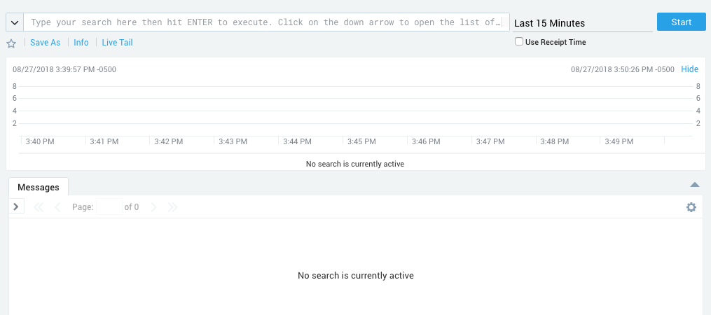
So that you may view your logs, Sumo Logic provides an interface containing a bar graph that breaks down the times when you received the most number of messages, a text field to enter a search, and a stream displaying all the matching logs. The most basic searches match a string against the body of the logs, but further refinement is easy. Sumo Logic keeps some metadata about your log sources by default, and keywords can be used in searches to help filter logs based on this data. These default categories are mostly intrinsic to the collector or are specific to the machine the collector is on (such as the id of the collector, the collector type, the hostname, etc.) but there is also a custom “source category” that can be entered by whoever set up the collectors to help group logs by function. Using categories to refine searches is simple and easy because the interface provides a tool-tip that suggests available categories, and this tool-tip can be expanded to list all available categories and all possible values.

Sumo Logic provides operators that allow you to perform parsing at search time so that you may create new columns in the log stream that contain the fields you are most interested in. These custom fields may also be used to further refine your search, allowing you to make effective use of identifying information within the logs themselves. Other than the parsing operators, Sumo Logic provides many other operations that can be performed during a search. Many operations are dedicated to working with strings, while others cast parsed fields into numbers and allow their manipulation. Additional operators allow you to group fields and change the output of the search, allowing you to focus on fields important to readers and hide additional fields used in the search. There are also miscellaneous operators such as count, which returns the number of results, or geo lookup which returns geographic coordinates based on an extracted IP address.

Individual log searches can be saved to a library for personal review or shared with others. These saved searches can be can be run manually or scheduled to run at intervals (you can even write a crontab expression if the fancy takes you and you’ve had your coffee) with the results of the search being emailed or sent through a web-hook. Combining this with thresholds (there are more/less than X results or some other condition), you can monitor your infrastructure and automatically alert someone when something goes awry.

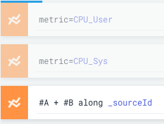
Viewing metrics is just as easy as viewing logs. The metric search interface contains a graph for displaying results, text field for entering the query, a tab for setting the axes, and a tab for filtering the results. The language for creating metric queries is the same as for writing log queries and differs only in the operators available. A successful query will return one or more time series, and most of the operators are dedicated to combining and transforming them by group (finding the min value or summing by hostname). Another difference from log searches is that once you have entered a query, a new query box will appear allowing you to run another query and add those time series to the graph as well. Queries can be referenced in future queries as well and you may perform mathematical operations to create new time series that are combinations of old ones. For example, this allows you to create a graph displaying total CPU usage by writing three queries: a system CPU usage query; a user CPU usage query; and a third query, which adds the previous two results together along hostnames.

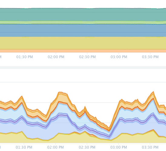
The metric search interface also includes a box for entering a log search. When combined with a log search, a bar graph will appear above the time series results to help correlate between trends in the time series and spikes in the number of matching logs.

Metric searches are saved and scheduled a little differently than log searches. Rather than being saved in the library, there is a metric alert screen that lists all previously created alerts, and it is from there that new metric searches can be created and saved (although a search created in the metric search interface can be automatically filled out in the metric alert interface). Metric alerts are a little more powerful than scheduled log searches because they can have multiple connections enabled at a time for their results (email, webhook, etc.), and have both critical and warning conditions.

Besides saving individual log searches for review later, searches of both types can be saved to panels in dashboards so that less experienced users can get a quick view of what’s going on across your systems without having to write their own searches. Dashboards normally operate in a mode where they must be refreshed manually to view new results, but they can also be operated in live mode where the panels are refreshed as results come in.

Currently, we use Sumo Logic to collect data originating from our applications and infrastructure. This data mostly takes the form of syslog logs, and metrics collected through installed Sumo Logic collectors.

The syslog data is collected in a central place in our infrastructure by a Sumo Logic collector running a syslog server. This is a hold-over from our old system and comes with a slight disadvantage; searching logs is slightly more complicated because as far as Sumo Logic is concerned, the logs come from only one source. This means that messages must contain identifying information, and searches must be written to parse this information. This is not much of an issue in practice because parsing is likely something a log search would contain anyway, but it adds an extra step to learn and increases the complexity of writing a search for a beginner. We have a battery of scheduled searches monitoring the data from our applications which alert based on the source and syslog severity level of the message as well as the presence of some keywords within the message body.

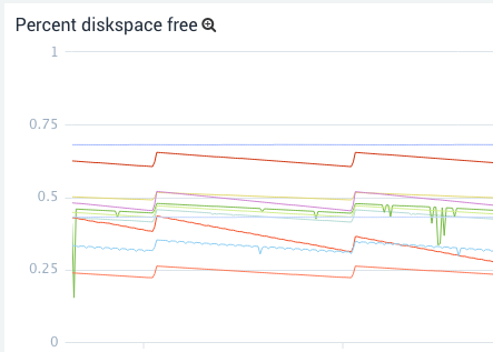
Metrics on the other hand, are ingested by collectors installed on each machine. This means that the metrics can be divided into appropriate categories and Sumo Logic collects metadata from every machine that makes searching easier. The installed collectors can be managed from Sumo Logic’s web interface, making it easy to change which metrics are collected and what category the collectors are in on a per-collector level. The rate at which metrics are collected is also controlled from the web interface, allowing you to control volumes if you are encroaching on your account limits. We had initially tried a solution where all metrics were being funnelled to a single collector running a graphite server but we found the convenience of managing each metric source from the web interface to be very helpful, (more so than for logs) and writing metric searches for this single collector was difficult. Most of our metric alerts monitor the free disk space on our servers and each alert is responsible for monitoring a specific class of device. For example, most of our boot devices have similar sizes and behave similarly so they can all be handled by one alert, while some devices are used for unique services and require their own alerts.

The data we currently collect isn’t of interest on a day-to-day level so currently Sumo Logic’s only role is to monitor and create PagerDuty alerts and Slack messages using web-hooks when something goes wrong. Compared to our old setup, Sumo Logic provides greater flexibility because it is much easier for a user to write their own search to quickly get a time series or log stream of interest, and our dependency on prebaked graphs and streams is diminished. Sumo Logic Dashboards also hold up to our old dashboards and have the advantage of combining graphed metrics with log streams and allowing users to extract a search from a panel so that they can tinker safely in a sandbox.

Our next step is to make better use of Sumo Logic’s analytic resources so that we might provide insight into areas of active research and development. This will require working with teams to identify new sources of data and come up with useful visualizations to help them make decisions relating to the performance of their systems. In expanding the amount of data we are collecting, it might be useful to reduce search time by splitting data up into distinct chunks using Sumo Logic’s partitioning features. Sumo Logic has also announced a logs-to-metrics feature which, when released, could be very valuable to us, as our logs contain numeric data that would be interesting to chart and monitor as if they were metrics.

Sumo Logic may initially appear complicated, but its interface is easy to use and can walk you through writing a query. Sumo Logic is a combined central collection point for logs and metrics, and offers flexibility and greater visibility into our data. If you are interested in using Sumo Logic or would like to know more details about all of its features checkout their website or the docs.