Scaling multi-output Gaussian process models with exact inference

19 Mar 2021

Author: Eric Perim, Wessel Bruinsma, and Will Tebbutt

In our previous post, we explained that multi-output Gaussian processes (MOGPs) are not fundamentally different from their single-output counterparts. We also introduced the Mixing Model Hierarchy (MMH), which is a broad class of MOGPs that covers several popular and powerful models from the literature. In this post, we will take a closer look at the central model from the MMH, the Instantaneous Linear Mixing Model (ILMM). We will discuss the linear algebra tricks that make inference in this model much cheaper than for general MOGPs. Then, we will take an alternative and more intuitive approach and use it as motivation for a yet better scaling model, the Orthogonal Instantaneous Linear Mixing Model (OILMM). Like most linear MOGPs, the OILMM represents data in a smaller-dimensional subspace; but contrary to most linear MOGPs, in practice the OILMM scales linearly with the dimensionality of this subspace, retaining exact inference.

Check out our previous post for a brief intro to MOGPs. We also recommend checking out the definition of the MMH from that post, but this post should be self-sufficient for those familiar with MOGPs. Some familiarity with linear algebra is also assumed. We start with the definition of the ILMM.

The Instantaneous Linear Mixing Model

Some data sets can exhibit a low-dimensional structure, where the data set presents an intrinsic dimensionality that is significantly lower than the dimensionality of the data. Imagine a data set consisting of coordinates in a 3D space. If the points in this data set form a single straight line, then the data is intrinsically one-dimensional, because each point can be represented by a single number once the supporting line is known. Mathematically, we say that the data lives in a lower dimensional (linear) subspace.

While this lower-dimensionality property may not be exactly true for most real data sets, many large real data sets frequently exhibit approximately low-dimensional structure, as discussed by Udell & Townsend (2019). In such cases, we can represent the data in a lower-dimensional space without losing a significant part of the information. There is a large field in statistics dedicated to identifying suitable lower-dimensional representations of data (e.g. Weinberger & Saul (2004)) and assessing their quality (e.g. Xia et al. (2017)). These dimensionality reduction techniques play an important role in computer vision (see Basri & Jacobs (2003) for an example), and in other fields (a paper by Markovsky (2008) contains an overview).

The Instantaneous Linear Mixing Model (ILMM) is a simple model that appears in many fields, e.g. machine learning (Bonilla et al. (2007) and Dezfouli et al. (2017)), signal processing (Osborne et al. (2008)), and geostatistics (Goovaerts (1997)). The model represents data in a lower-dimensional linear subspace—not unlike PCA— which implies the model’s covariance matrix is low-rank. As we will discuss in the next sections, this low-rank structure can be exploited for efficient inference. In the ILMM, the observations are described as a linear combination of latent processes (i.e. unobserved stochastic processes), which are modelled as single-output GPs.

If we denote our observations as \(y\), the ILMM models the data according to the following generative model: \(y(t) \cond x, H = Hx(t) + \epsilon\). Here, \(y(t) \cond x, H\) is used to denote the value of \(y(t)\) given a known \(H\) and \(x(t)\), \(H\) is a matrix of weights, which we call the mixing matrix, \(\epsilon\) is Gaussian noise, and \(x(t)\) represents the (time-dependent) latent processes, described as independent GPs—note that we use \(x\) here to denote an unobserved (latent) stochastic process, not an input, which is represented by \(t\). Using an ILMM with \(m\) latent processes to model \(p\) outputs, \(y(t)\) is \(p\)-dimensional, \(x(t)\) is \(m\)-dimensional, and \(H\) is a \(p \times m\) matrix. Since the latent processes are GPs, and Gaussian random variables are closed under linear combinations, \(y(t)\) is also a GP. This means that the usual closed-form formulae for inference in GPs can be used. However, naively computing these formulae is not computationally efficient, because a large covariance matrix has to be inverted, which is a significant bottleneck. In the next section we discuss tricks to speed up this inversion.

Leveraging the matrix inversion lemma

When working with GPs, the computational bottleneck is typically the inversion of the covariance matrix over the training input locations. For the case of the ILMM, observing \(p\) outputs, each at \(n\) input locations, we require the inversion of an \(np \times np\) matrix. This operation quickly becomes computationally intractable. What sets the ILMM apart from the general MOGP case is that the covariance matrices generated via an ILMM have some structure that can be exploited.

There is a useful and widely used result from linear algebra that allows us to exploit this structure, known as the matrix inversion lemma (also known as the Sherman–Morrison–Woodbury formula, or simply as the Woodbury matrix formula). This lemma comes in handy whenever we want to invert a matrix that can be written as the sum of a low-rank matrix and a diagonal one.¹ Whereas typically the inversion of such matrices scales with the size of the matrix, the lemma cleverly allows the inversion operation to scale with the rank of the low-rank matrix instead. Therefore, if the rank of the low-rank matrix is much smaller than the size of the matrix, the lemma can enable significant computational speed-ups. We can show that the covariance of the ILMM can be written as a sum of a low-rank and diagonal matrix, which means that the matrix inversion lemma can be applied.

For an ILMM that has \(n\) observations for each of \(p\) outputs and uses \(m\) latent processes, the covariance matrix has size \(np \times np\), but the low-rank part has rank \(nm \times nm\). Thus, by choosing an \(m\) that is smaller than \(p\) and using the matrix inversion lemma, we can effectively decrease the memory and time costs associated with the matrix inversion.

This is not the first time we leverage the matrix inversion lemma to make computations more efficient, see our post on linear models from a GP point of view for another example. The ubiquity of models that represent data in lower-dimensional linear subspaces makes the use of this lemma widespread. However, this approach requires careful application of linear algebra tricks, and obfuscates the reason why it is even possible to get such a speed-up. In the next section we show an alternative view, which is more intuitive and leads to the same performance improvements.

An alternative formulation

Instead of focusing on linear algebra tricks, let’s try to understand why we can even reduce the complexity of the inversion. The ILMM, as a general GP, scales poorly with the number of observations; and the larger the number of outputs, the larger the number of observations. However, the ILMM makes the modelling assumption that the observations can be represented in a lower-dimensional space. Intuitively, that means that every observation contains a lot of redundant information, because it can be summarised by a much lower-dimensional representation. If it were possible to somehow extract these lower-dimensional representations and use them as observations instead, then that could lead to very appealing computational gains. The challenge here is that we don’t have access to the lower-dimensional representations, but we can try to estimate them.

Recall that the ILMM is a probabilistic model that connects every observation \(y(t)\) to a set of latent, unobserved variables \(x(t)\), defining the lower-dimensional representation. It is this lower-dimensional \(x(t)\) that we want to estimate. A natural choice is to find the maximum likelihood estimate (MLE) \(T(y(t))\) of \(x(t)\) given the observations \(y(t)\):

\[\begin{equation} T(y(t)) = \underset{x(t)}{\mathrm{argmax}} \, p(y(t) \cond x(t)). \end{equation}\]

The solution to the equation above is \(T = (H^\top \Sigma^{-1} H)^{-1} H^\top \Sigma^{-1}\) (see prop. 2 of appendix D from Bruinsma et al. (2020)), where \(H\) is the mixing matrix, and \(\Sigma\) is the noise covariance.

The advantage of working with \(Ty(t)\) instead of with \(y(t)\) is that \(y(t)\) comprises \(p\) outputs, while \(Ty(t)\) presents only \(m\) outputs. Thus, conditioning on \(Ty(t)\) is computationally cheaper because \(m < p\). When conditioning on \(n\) observations, this approach brings the memory cost from \(\mathcal{O}(n^2p^2)\) to \(\mathcal{O}(n^2m^2)\), and the time cost from \(\mathcal{O}(n^3p^3)\) to \(\mathcal{O}(n^3m^3)\).² These savings are identical to those we get by using the matrix inversion lemma, as discussed in the previous section.

In general, we cannot arbitrarily transform observations and use the resulting transformed data as observations instead. We must show that our proposed procedure is valid, that conditioning on \(Ty(t)\) is equivalent to conditioning on \(y(t)\). We do this showing that (see Bruinsma et al. (2020)),³ under the ILMM, \(Ty(t)\) is a sufficient statistic for \(x(t)\) given \(y\)—and this is only possible because of the particular structure of the ILMM.

A sufficient statistic \(T(y)\) is a function of the data which is defined with respect to a probabilistic model, \(p(y \cond \theta)\), and an associated unknown parameter \(\theta\). When a statistic is sufficient, it means that computing it over a set of observations, \(y\), provides us with all the information about \(\theta\) that can be extracted from those observations (under that probabilistic model). Thus, there is no other quantity we can compute over \(y\) that will increase our knowledge of \(\theta\). Formally, that is to say that \(p(\theta \cond y) = p(\theta \cond T(y))\). For the ILMM, as \(Ty(t)\) is a sufficient statistic for \(x(t)\), we have that \(p(x(t) \cond y(t)) = p(x(t) \cond Ty(t))\). This property guarantees that the procedure of conditioning the model on the summary of the observations is mathematically valid.

The choice of \(m < p\) is exactly the choice of imposing a low-rank structure onto the model; and the lower the rank (controlled by \(m\), the number of latent processes), the more parsimonious is \(Ty\), the summary of our observations.

Besides being more intuitive, this approach based on the sufficient statistic makes it easy to see how introducing a simple constraint over the mixing matrix \(H\) will allow us to scale the model even further, and obtain linear scaling on the number of latent processes, \(m\).⁴ That’s what we discuss next.

The Orthogonal Instantaneous Linear Mixing Model

Although the ILMM scales much better than a general MOGP, the ILMM still has a cubic (quadratic) scaling on \(m\) for time (memory), which quickly becomes intractable for large systems. We therefore want to identify a subset of the ILMMs that scale even more favourably. We show that a very simple restriction over the mixing matrix \(H\) can lead to linear scaling on \(m\) for both time and memory. We call this model the Orthogonal Instantaneous Linear Mixing Model (OILMM). The plots below show a comparison of the time and memory scaling for the ILMM vs the OILMM as \(m\) grows.

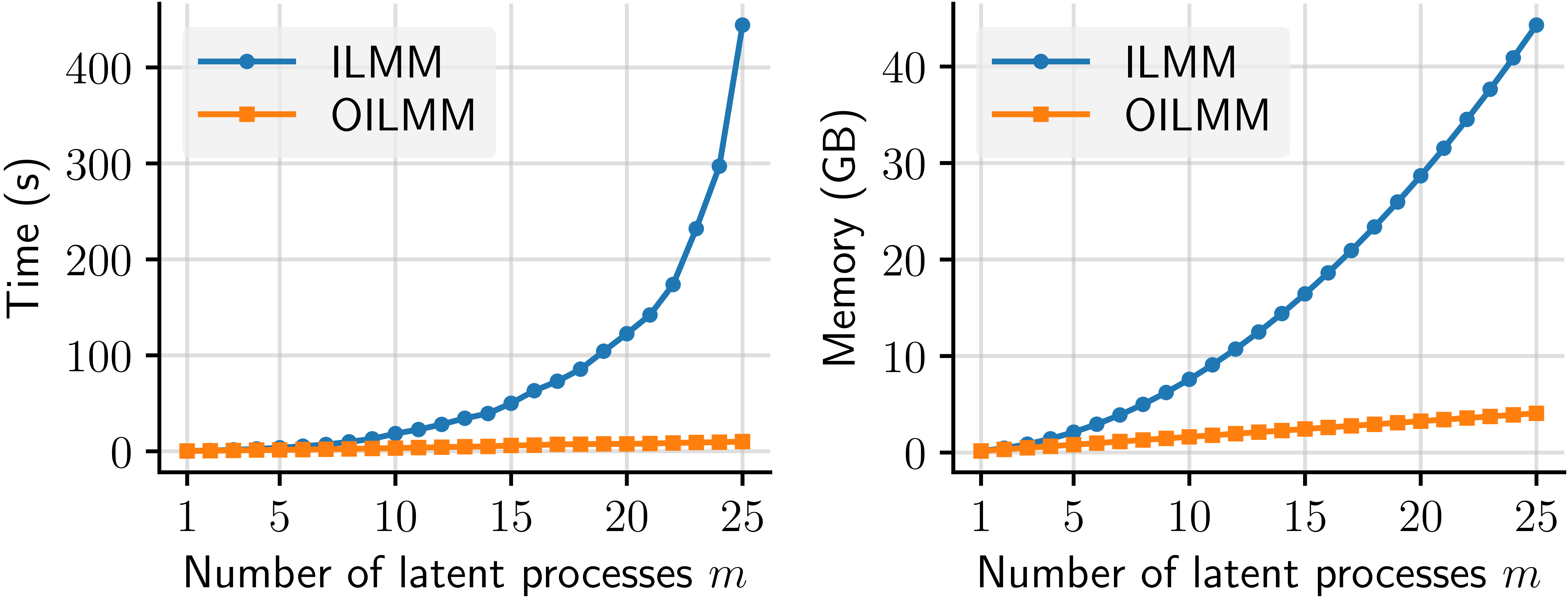Figure 1: Runtime (left) and memory usage (right) of the ILMM and OILMM for computing the evidence of \(n = 1500\) observations for \(p = 200\) outputs.

Let’s return to the definition of the ILMM, as discussed in the first section: \(y(t) \cond x(t), H = Hx(t) + \epsilon(t)\). Because \(\epsilon(t)\) is Gaussian noise, we can write that \(y(t) \cond x(t), H \sim \mathrm{GP}(Hx(t), \delta_{tt'}\Sigma)\), where \(\delta_{tt'}\) is the Kronecker delta. Because we know that \(Ty(t)\) is a sufficient statistic for \(x(t)\) under this model, we know that \(p(x \cond y(t)) = p(x \cond Ty(t))\). Then what is the distribution of \(Ty(t)\)? A simple calculation gives \(Ty(t) \cond x(t), H \sim \mathrm{GP}(THx(t), \delta_{tt'}T\Sigma T^\top)\). The crucial thing to notice here is that the summarised observations \(Ty(t)\) only couple the latent processes \(x\) via the noise matrix \(T\Sigma T^\top\). If that matrix were diagonal, then observations would not couple the latent processes, and we could condition each of them individually, which is much more computationally efficient.

This is the insight for the Orthogonal Instantaneous Linear Mixing Model (OILMM). If we let \(\Sigma = \sigma^2I_p\), then it can be shown that \(T\Sigma T^\top\) is diagonal if and only if the columns of \(H\) are orthogonal (Prop. 6 from the paper by Bruinsma et al. (2020)), which means that \(H\) can be written as \(H = US^{1/2}\), with \(U\) a matrix of orthonormal columns, and \(S > 0\) diagonal. Because the columns of \(H\) are orthogonal, we name the OILMM orthogonal. In summary: by restricting the columns of the mixing matrix in an ILMM to be orthogonal, we make it possible to treat each latent process as an independent, single-output GP problem.

The result actually is a bit more general: we can allow any observation noise of the form \(\sigma^2I_p + H D H^\top\), with \(D>0\) diagonal. Thus, it is possible to have a non-diagonal noise matrix, i.e., noise that is correlated across different outputs, and still be able to decouple the latent processes and retain all computational gains from the OILMM (which we discuss next).

Computationally, the OILMM approach allows us to go from a cost of \(\mathcal{O}(n^3m^3)\) in time and \(\mathcal{O}(n^2m^2)\) in memory, for a regular ILMM, to \(\mathcal{O}(n^3m)\) in time and \(\mathcal{O}(n^2m)\) in memory. This is because now the problem reduces to \(m\) independent single-output GP problems.⁵ The figure below explains the inference process under the ILMM and the OILMM, with the possible paths and the associated costs.

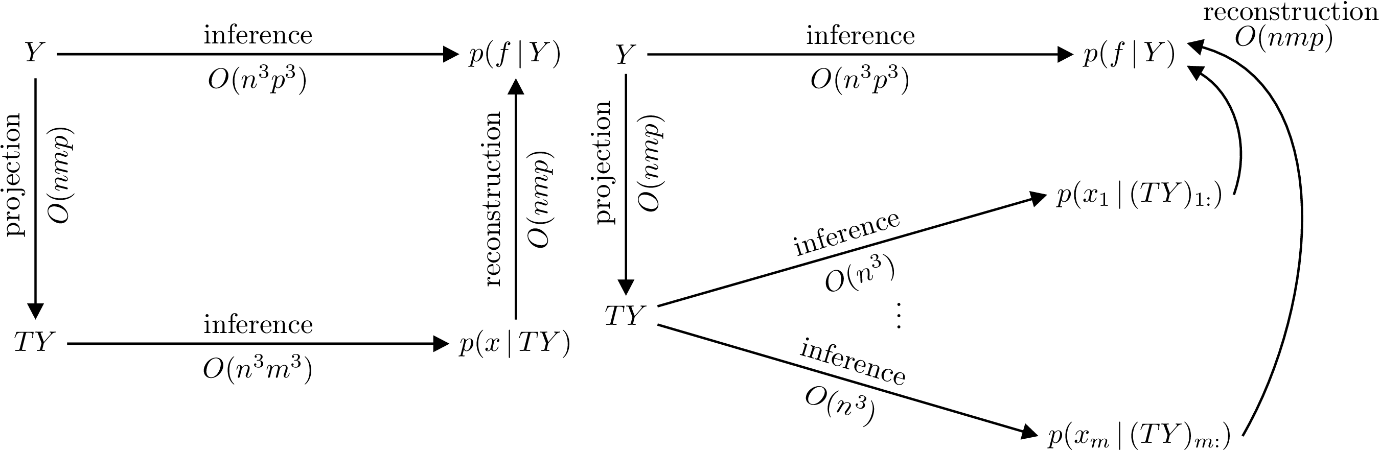Figure 2: Commutative diagrams depicting that conditioning on \(Y\) in the ILMM (left) and OILMM (right) is equivalent to conditioning respectively on \(TY\) and independently every \(x_i\) on \((TY)_{i:}\), but yield different computational complexities. The reconstruction costs assume computation of the marginals.

If we take the view of an (O)ILMM representing every data point \(y(t)\) via a set of basis vectors \(h_1, \ldots, h_m\) (the columns of the mixing matrix) and a set of time-dependent coefficients \(x_1(t), \ldots, x_m(t)\) (the latent processes), the difference between an ILMM and an OILMM is that in the latter the coordinate system is chosen to be orthogonal, as is common practice in most fields. This insight is illustrated below.

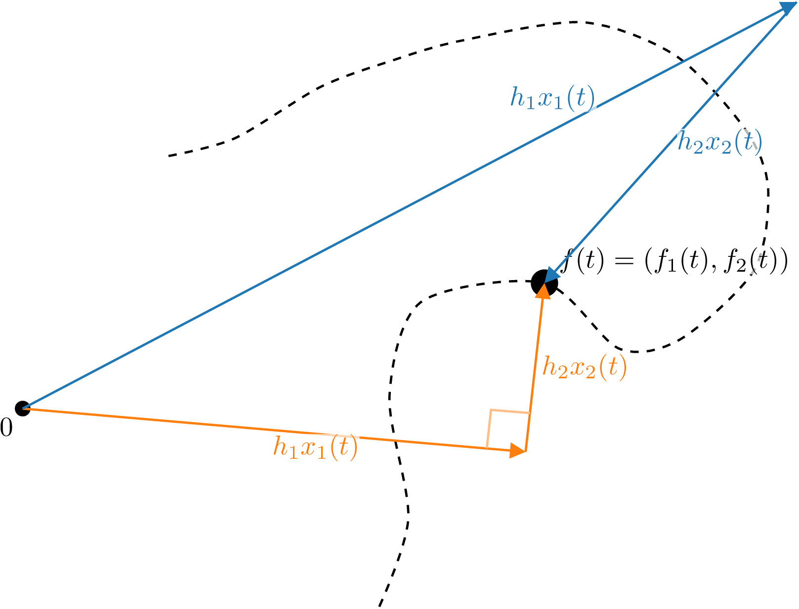Figure 3: Illustration of the difference between the ILMM and OILMM. The trajectory of a particle (dashed line) in two dimensions is modelled by the ILMM (blue) and OILMM (orange). The noise-free position \(f(t)\) is modelled as a linear combination of basis vectors \(h_1\) and \(h_2\) with coefficients \(x_1(t)\) and \(x_2(t)\) (two independent GPs). In the OILMM, the basis vectors \(h_1\) and \(h_2\) are constrained to be orthogonal; in the ILMM, \(h_1\) and \(h_2\) are unconstrained.

Another important difference between a general ILMM and an OILMM is that, while in both cases the latent processes are independent a priori, only for an OILMM they remain so a posteriori. Besides the computational gains we already mentioned, this property also improves interpretability as the posterior latent marginal distributions can be inspected (and plotted) independently. In comparison, inspecting only the marginal distributions in a general ILMM would neglect the correlations between them, obscuring the interpretation.

Finally, the fact that an OILMM problem is just really a set of single-output GP problems makes the OILMM immediately compatible with any single-output GP approach. This allows us to trivially use powerful approaches, like sparse GPs (as detailed in the paper by Titsias (2009)), or state-space approximations (as presented in the freely available book by Särkkä & Solin), for scaling to extremely large data sets. We have illustrated this by using the OILMM, combined with state-space approximations, to model 70 million data points (see Bruinsma et al. (2020) for details).

Conclusion

In this post we have taken a deeper look into the Instantaneous Linear Mixing Model (ILMM), a widely used multi-output GP (MOGP) model which stands at the base of the Mixing Model Hierarchy (MMH)—which was described in detail in our previous post. We discussed how the matrix inversion lemma can be used to make computations much more efficient. We then showed an alternative but equivalent (and more intuitive) view based on a sufficient statistic for the model. This alternative view gives us a better understanding on why and how these computational gains are possible.

From the sufficient statistic formulation of the ILMM we showed how a simple constraint over one of the model parameters can decouple the MOGP problem into a set of independent single-output GP problems, greatly improving scalability. We call this model the Orthogonal Instantaneous Linear Mixing Model (OILMM), a subset of the ILMM.

In the next and last post in this series, we will discuss implementation details of the OILMM and show some of our implementations in Julia and in Python.

Notes