19 Jan 2021
Author: Wessel Bruinsma and James Requeima
Cross-posted at wesselb.github.io.
A linear model prescribes a linear relationship between inputs and outputs.
Linear models are amongst the simplest of models, but they are ubiquitous across science.
A linear model with Gaussian distributions on the coefficients forms one of the simplest instances of a Gaussian process.
In this post, we will give a brief introduction to linear models from a Gaussian process point of view.
We will see how a linear model can be implemented with Gaussian process probabilistic programming using Stheno, and how this model can be used to denoise noisy observations.
(Disclosure: Will Tebbutt and Wessel are the authors of Stheno;
Will maintains a Julia version.)
In short, probabilistic programming is a programming paradigm that brings powerful probabilistic models to the comfort of your programming language, which often comes with tools to automatically perform inference (make predictions).
We will also use JAX’s just-in-time compiler to make our implementation extremely efficient.
Linear Models from a Gaussian Process Point of View
Consider a data set \((x_i, y_i)_{i=1}^n \subseteq \R \times \R\) consisting of \(n\) real-valued input–output pairs.
Suppose that we wish to estimate a linear relationship between the inputs and outputs:
\[\label{eq:ax_b}
y_i = a \cdot x_i + b + \e_i,\]
where \(a\) is an unknown slope, \(b\) is an unknown offset, and \(\e_i\) is some error/noise associated with the observation \(y_i\).
To implement this model with Gaussian process probabilistic programming, we need to cast the problem into a functional form.
This means that we will assume that there is some underlying, random function \(y \colon \R \to \R\) such that the observations are evaluations of this function: \(y_i = y(x_i)\).
The model for the random function \(y\) will embody the structure of the linear model \eqref{eq:ax_b}.
This may sound hard, but it is not difficult at all.
We let the random function \(y\) be of the following form:
\[\label{eq:ax_b_functional}
y(x) = a(x) \cdot x + b(x) + \e(x)\]
where \(a\colon \R \to \R\) is a random constant function.
An example of a constant function \(f\) is \(f(x) = 5\).
Random means that the value \(5\) is not fixed, but modelled with a random value drawn from some probability distribution, because we don’t know the true value.
We let \(b\colon \R \to \R\) also be a random constant function, and \(\e\colon \R \to \R\) a random noise function.
Do you see the similarities between \eqref{eq:ax_b} and \eqref{eq:ax_b_functional}?
If all that doesn’t fully make sense, don’t worry; things should become more clear as we implement the model.
To model random constant functions and random noise functions, we will use Stheno, which is a Python library for Gaussian process modelling.
We also have a Julia version, but in this post we’ll use the Python version.
To install Stheno, run the command
pip install --upgrade --upgrade-strategy eager stheno
In Stheno, a Gaussian process can be created with GP(kernel), where kernel is the so-called kernel or covariance function of the Gaussian process.
The kernel determines the properties of the function that the Gaussian process models.
For example, the kernel EQ() models smooth functions, and the kernel Matern12() models functions that look jagged.
See the kernel cookbook for an overview of commonly used kernels and the documentation of Stheno for the corresponding classes.
For constant functions, you can set the kernel to simply a constant, for example 1, which then models the constant function with a value drawn from \(\mathcal{N}(0, 1)\). (By default, in Stheno, all means are zero; but, if you like, you can also set a mean.)
Let’s start out by creating a Gaussian process for the random constant function \(a(x)\) that models the slope.
>>> from stheno import GP

>>> a = GP(1)

>>> a
GP(0, 1)
You can see how the Gaussian process looks by simply sampling from it.
To sample from the Gaussian process a at some inputs x, evaluate it at those inputs, a(x), and call the method sample: a(x).sample().
This shows that you can really think of a Gaussian process just like you think of a function:
pass it some inputs to get (the model for) the corresponding outputs.
>>> x = np.linspace(0, 10, 100)

>>> plt.plot(x, a(x).sample(20)); plt.show()
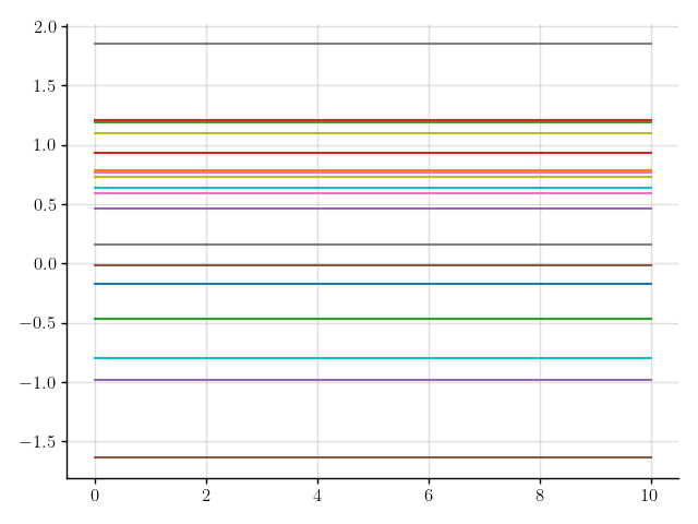 Figure 1: Samples of a Gaussian process that models a constant function.
We’ve sampled a bunch of constant functions.
Sweet!
The next step in the model \eqref{eq:ax_b_functional} is to multiply the slope function \(a(x)\) by \(x\).
To multiply a by \(x\), we multiply a by the function lambda x: x, which casts also \(x\) as a function:
>>> f = a * (lambda x: x)

>>> f
GP(0, <lambda>)
This will give rise to functions like \(x \mapsto 0.1x\) and \(x \mapsto -0.4x\), depending on the value that \(a(x)\) takes.
>>> plt.plot(x, f(x).sample(20)); plt.show()
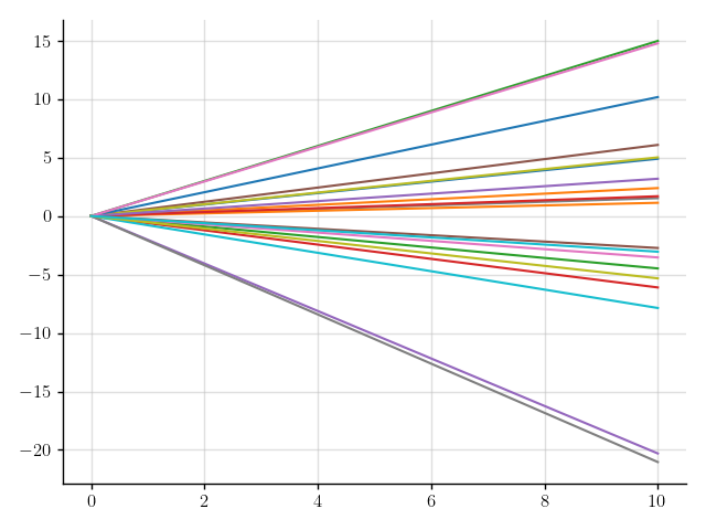 Figure 2: Samples of a Gaussian process that models functions with a random slope.
This is starting to look good!
The only ingredient that is missing is an offset.
We model the offset just like the slope, but here we set the kernel to 10 instead of 1, which models the offset with a value drawn from \(\mathcal{N}(0, 10)\).
>>> b = GP(10)

>>> f = a * (lambda x: x) + b
AssertionError: Processes GP(0, <lambda>) and GP(0, 10 * 1) are associated to different measures.
Something went wrong.
Stheno has an abstraction called measures, where only GPs that are part of the same measure can be combined into new GPs;
the abstraction of measures is there to keep things safe and tidy.
What goes wrong here is that a and b are not part of the same measure.
Let’s explicitly create a new measure and attach a and b to it.
>>> from stheno import Measure

>>> prior = Measure()

>>> a = GP(1, measure=prior)

>>> b = GP(10, measure=prior)

>>> f = a * (lambda x: x) + b

>>> f
GP(0, <lambda> + 10 * 1)
Let’s see how samples from f look like.
>>> plt.plot(x, f(x).sample(20)); plt.show()
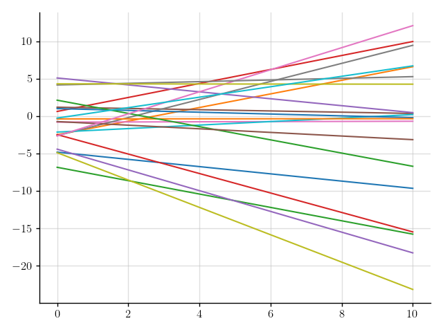 Figure 3: Samples of a Gaussian process that models linear functions.
Perfect!
We will use f as our linear model.
In practice, observations are corrupted with noise.
We can add some noise to the lines in Figure 3 by adding a Gaussian process that models noise.
You can construct such a Gaussian process by using the kernel Delta(), which models the noise with independent \(\mathcal{N}(0, 1)\) variables.
>>> from stheno import Delta

>>> noise = GP(Delta(), measure=prior)

>>> y = f + noise

>>> y
GP(0, <lambda> + 10 * 1 + Delta())

>>> plt.plot(x, y(x).sample(20)); plt.show()
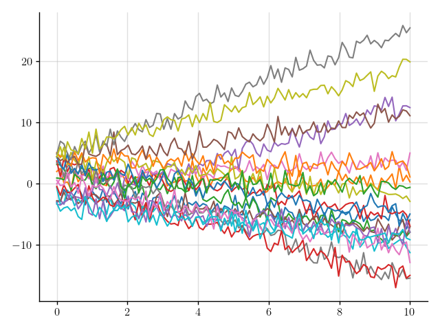 Figure 4: Samples of a Gaussian process that models noisy linear functions.
That looks more realistic, but perhaps that’s a bit too much noise.
We can tune down the amount of noise, for example, by scaling noise by 0.5.
>>> y = f + 0.5 * noise

>>> y
GP(0, <lambda> + 10 * 1 + 0.25 * Delta())

>>> plt.plot(x, y(x).sample(20)); plt.show()
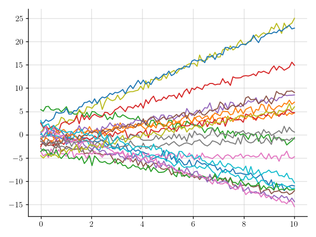 Figure 5: Samples of a Gaussian process that models noisy linear functions.
Much better.
To summarise, our linear model is given by
prior = Measure()

a = GP(1, measure=prior)            # Model for slope
b = GP(10, measure=prior)           # Model for offset
f = a * (lambda x: x) + b           # Noiseless linear model

noise = GP(Delta(), measure=prior)  # Model for noise
y = f + 0.5 * noise                 # Noisy linear model
We call a program like this a Gaussian process probabilistic program (GPPP).
Let’s generate some noisy synthetic data, (x_obs, y_obs), that will make up an example data set \((x_i, y_i)_{i=1}^n\).
We also save the observations without noise added—f_obs—so we can later check how good our predictions really are.
>>> x_obs = np.linspace(0, 10, 50_000)

>>> f_obs = 0.8 * x_obs - 2.5

>>> y_obs = f_obs + 0.5 * np.random.randn(50_000)

>>> plt.scatter(x_obs, y_obs); plt.show()
 Figure 6: Some observations.
We will see next how we can fit our model to this data.
Inference in Linear Models
Suppose that we wish to remove the noise from the observations in Figure 6.
We carefully phrase this problem in terms of our GPPP:
the observations y_obs are realisations of the noisy linear model y at x_obs—realisations of y(x_obs)—and we wish to make predictions for the noiseless linear model f at x_obs—predictions for f(x_obs).
In Stheno, we can make predictions based on observations by conditioning the measure of the model on the observations.
In our GPPP, the measure is given by prior, so we aim to condition prior on the observations y_obs for y(x_obs).
Mathematically, this process of incorporating information by conditioning happens through Bayes’ rule.
Programmatically, we first make an Observations object, which represents the information—the observations—that we want to incorporate, and then condition prior on this object:
>>> from stheno import Observations

>>> obs = Observations(y(x_obs), y_obs)

>>> post = prior.condition(obs)
You can also more concisely perform these two steps at once, as follows:
>>> post = prior | (y(x_obs), y_obs)
This mimics the mathematical notation used for conditioning.
With our updated measure post, which is often called the posterior measure, we can make a prediction for f(x_obs) by passing f(x_obs) to post:
>>> pred = post(f(x_obs))

>>> pred.mean
<dense matrix: shape=50000x1, dtype=float64
 mat=[[-2.498]
      [-2.498]
      [-2.498]
      ...
      [ 5.501]
      [ 5.502]
      [ 5.502]]>

>>> pred.var
<low-rank matrix: shape=50000x50000, dtype=float64, rank=2
 left=[[1.e+00 0.e+00]
       [1.e+00 2.e-04]
       [1.e+00 4.e-04]
       ...
       [1.e+00 1.e+01]
       [1.e+00 1.e+01]
       [1.e+00 1.e+01]]
 middle=[[ 2.001e-05 -2.995e-06]
         [-2.997e-06  6.011e-07]]
 right=[[1.e+00 0.e+00]
        [1.e+00 2.e-04]
        [1.e+00 4.e-04]
        ...
        [1.e+00 1.e+01]
        [1.e+00 1.e+01]
        [1.e+00 1.e+01]]>
The prediction pred is a multivariate Gaussian distribution with a particular mean and variance, which are displayed above.
You should view post as a function that assigns a probability distribution—the prediction—to every part of our GPPP, like f(x_obs).
Note that the variance of the prediction is a massive matrix of size 50k \(\times\) 50k.
Under the hood, Stheno uses structured representations for matrices to compute and store matrices in an efficient way.
Let’s see how the prediction pred for f(x_obs) looks like.
The prediction pred exposes the method marginals that conveniently computes the mean and associated lower and upper error bounds for you.
>>> mean, error_bound_lower, error_bound_upper  = pred.marginals()

>>> mean
array([-2.49818708, -2.49802708, -2.49786708, ...,  5.50148996,
        5.50164996,  5.50180997])

>>> error_bound_upper - error_bound_lower
array([0.01753381, 0.01753329, 0.01753276, ..., 0.01761883, 0.01761935,
       0.01761988])
The error is very small—on the order of \(10^{-2}\)—which means that Stheno predicted f(x_obs) with high confidence.
>>> plt.scatter(x_obs, y_obs); plt.plot(x_obs, mean); plt.show()
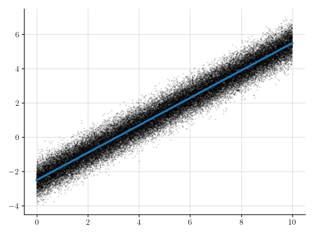 Figure 7: Mean of the prediction (blue line) for the denoised observations.
The blue line in Figure 7 shows the mean of the predictions.
This line appears to nicely pass through the observations with the noise removed.
But let’s see how good the predictions really are by comparing to f_obs, which we previously saved.
>>> f_obs - mean
array([-0.00181292, -0.00181292, -0.00181292, ..., -0.00180997,
       -0.00180997, -0.00180997])

>>> np.mean((f_obs - mean) ** 2)  # Compute the mean square error.
3.281323087544209e-06
That’s pretty close!
Not bad at all.
We wrap up this section by encapsulating everything that we’ve done so far in a function linear_model_denoise, which denoises noisy observations from a linear model:
def linear_model_denoise(x_obs, y_obs):
    prior = Measure()
    a = GP(1, measure=prior)            # Model for slope
    b = GP(10, measure=prior)           # Model for offset
    f = a * (lambda x: x) + b           # Noiseless linear model
    noise = GP(Delta(), measure=prior)  # Model for noise
    y = f + 0.5 * noise                 # Noisy linear model

    post = prior | (y(x_obs), y_obs)    # Condition on observations.
    pred = post(f(x_obs))               # Make predictions.
    return pred.marginals()             # Return the mean and associated error bounds.
>>> linear_model_denoise(x_obs, y_obs)
(array([-2.49818708, -2.49802708, -2.49786708, ...,  5.50148996,
        5.50164996,  5.50180997]), array([-2.50695399, -2.50679372, -2.50663346, ...,  5.49268055,
        5.49284029,  5.49300003]), array([-2.48942018, -2.48926044, -2.4891007 , ...,  5.51029937,
        5.51045964,  5.51061991]))

>>> %timeit linear_model_denoise(x_obs, y_obs)
233 ms ± 12.6 ms per loop (mean ± std. dev. of 7 runs, 1 loop each)
To denoise 50k observations, linear_model_denoise takes about 250 ms.
Not terrible, but we can do much better, which is important if we want to scale to larger numbers of observations.
In the next section, we will make this function really fast.
Making Inference Fast
To make linear_model_denoise fast, firstly, the linear algebra that happens under the hood when linear_model_denoise is called should be simplified as much as possible.
Fortunately, this happens automatically, due to the structured representation of matrices that Stheno uses.
For example, when making predictions with Gaussian processes, the main computational bottleneck is usually the construction and inversion of y(x_obs).var, the variance associated with the observations:
>>> y(x_obs).var
<Woodbury matrix: shape=50000x50000, dtype=float64
 diag=<diagonal matrix: shape=50000x50000, dtype=float64
       diag=[0.25 0.25 0.25 ... 0.25 0.25 0.25]>
 lr=<low-rank matrix: shape=50000x50000, dtype=float64, rank=2
     left=[[1.e+00 0.e+00]
           [1.e+00 2.e-04]
           [1.e+00 4.e-04]
           ...
           [1.e+00 1.e+01]
           [1.e+00 1.e+01]
           [1.e+00 1.e+01]]
     middle=[[10.  0.]
             [ 0.  1.]]
     right=[[1.e+00 0.e+00]
            [1.e+00 2.e-04]
            [1.e+00 4.e-04]
            ...
            [1.e+00 1.e+01]
            [1.e+00 1.e+01]
            [1.e+00 1.e+01]]>>
Indeed observe that this matrix has particular structure:
it is a sum of a diagonal and a low-rank matrix.
In Stheno, the sum of a diagonal and a low-rank matrix is called a Woodbury matrix, because the Sherman–Morrison–Woodbury formula can be used to efficiently invert it.
Let’s see how long it takes to construct y(x_obs).var and then invert it.
We invert y(x_obs).var using LAB, which is automatically installed alongside Stheno and exposes the API to efficiently work with structured matrices.
>>> import lab as B

>>> %timeit B.inv(y(x_obs).var)
28.5 ms ± 1.69 ms per loop (mean ± std. dev. of 7 runs, 10 loops each)
That’s only 30 ms! Not bad, for such a big matrix. Without exploiting structure, a 50k \(\times\) 50k matrix takes 20 GB of memory to store and about an hour to invert.
Secondly, we would like the code implemented by linear_model_denoise to be as efficient as possible.
To achieve this, we will use JAX to compile linear_model_denoise with XLA, which generates blazingly fast code.
We start out by importing JAX and loading the JAX extension of Stheno.
>>> import jax

>>> import jax.numpy as jnp

>>> import stheno.jax  # JAX extension for Stheno
We use JAX’s just-in-time (JIT) compiler jax.jit to compile linear_model_denoise:
>>> linear_model_denoise_jitted = jax.jit(linear_model_denoise)
Let’s see what happens when we run linear_model_denoise_jitted.
We must pass x_obs and y_obs as JAX arrays to use the compiled version.
>>> linear_model_denoise_jitted(jnp.array(x_obs), jnp.array(y_obs))
Invalid argument: Cannot bitcast types with different bit-widths: F64 => S32.
Oh no!
What went wrong is that the JIT compiler wasn’t able to deal with the complicated control flow from the automatic linear algebra simplifications.
Fortunately, there is a simple way around this:
we can run the function once with NumPy to see how the control flow should go, cache that control flow, and then use this cache to run linear_model_denoise with JAX.
Sounds complicated, but it’s really just a bit of boilerplate:
>>> import lab as B

>>> control_flow_cache = B.ControlFlowCache()

>>> control_flow_cache
<ControlFlowCache: populated=False>
Here populated=False means that the cache is not yet populated.
Let’s populate it by running linear_model_denoise once with NumPy:
>>> with control_flow_cache:
        linear_model_denoise(x_obs, y_obs)

>>> control_flow_cache
<ControlFlowCache: populated=True>
We now construct a compiled version of linear_model_denoise that uses the control flow cache:
@jax.jit
def linear_model_denoise_jitted(x_obs, y_obs):
    with control_flow_cache:
        return linear_model_denoise(x_obs, y_obs)
>>> linear_model_denoise_jitted(jnp.array(x_obs), jnp.array(y_obs))
(DeviceArray([-2.4981871 , -2.4980271 , -2.49786709, ...,  5.50149004,
              5.50165005,  5.50181005], dtype=float64), DeviceArray([-2.5069514 , -2.50679114, -2.50663087, ...,  5.4927699 ,
              5.49292964,  5.49308938], dtype=float64), DeviceArray([-2.4894228 , -2.48926306, -2.48910332, ...,  5.51021019,
              5.51037046,  5.51053072], dtype=float64))
Nice!
Let’s see how much faster linear_model_denoise_jitted is:
>>> %timeit linear_model_denoise(x_obs, y_obs)
233 ms ± 12.6 ms per loop (mean ± std. dev. of 7 runs, 1 loop each)

>>> %timeit linear_model_denoise_jitted(jnp.array(x_obs), jnp.array(y_obs))
1.63 ms ± 16.5 µs per loop (mean ± std. dev. of 7 runs, 1000 loops each)
The compiled function linear_model_denoise_jitted only takes 2 ms to denoise 50k observations!
Compared to linear_model_denoise, that’s a speed-up of two orders of magnitude.
Conclusion
We’ve seen how a linear model can be implemented with a Gaussian process probabilistic program (GPPP) using Stheno.
Stheno allows us to focus on model construction, and takes away the distraction of the technicalities that come with making predictions.
This flexibility, however, comes at the cost of some complicated machinery that happens in the background, such as structured representations of matrices.
Fortunately, we’ve seen that this overhead can be completely avoided by compiling your program using JAX, which can result in extremely efficient implementations.
To close this post and to warm you up for what’s further possible with Gaussian process probabilistic programming using Stheno, the linear model that we’ve built can easily be extended to, for example, include a quadratic term:
def quadratic_model_denoise(x_obs, y_obs):
    prior = Measure()
    a = GP(1, measure=prior)            # Model for slope
    b = GP(1, measure=prior)            # Model for coefficient of quadratic term
    c = GP(10, measure=prior)           # Model for offset
    # Noiseless quadratic model
    f = a * (lambda x: x) + b * (lambda x: x ** 2) + c
    noise = GP(Delta(), measure=prior)  # Model for noise
    y = f + 0.5 * noise                 # Noisy quadratic model

    post = prior | (y(x_obs), y_obs)    # Condition on observations.
    pred = post(f(x_obs))               # Make predictions.
    return pred.marginals()             # Return the mean and associated error bounds.
To use Gaussian process probabilistic programming for your specific problem, the main challenge is to figure out which model you need to use.
Do you need a quadratic term?
Maybe you need an exponential term!
But, using Stheno, implementing the model and making predictions should then be simple.
04 Dec 2020
Author: Letif Mones
Although governed by simple physical laws, power grids are among the most complex human-made systems.
The main source of the complexity is the large number of components of the power systems that interact with each other: one needs to maintain a balance between power injections and withdrawals while satisfying certain physical, economic, and environmental conditions.
For instance, a central task of daily planning and operations of electricity grid operators is to dispatch generation in order to meet demand at minimum cost, while respecting reliability and security constraints.
These tasks require solving a challenging constrained optimization problem, often referred to as some form of optimal power flow (OPF).
In a series of two blog posts, we are going to discuss the basics of power flow and optimal power flow problems.
In this first post, we focus on the most important component of OPF: the power flow (PF) equations.
For this, first we introduce some basic definitions of power grids and AC circuits, then we define the power flow problem.
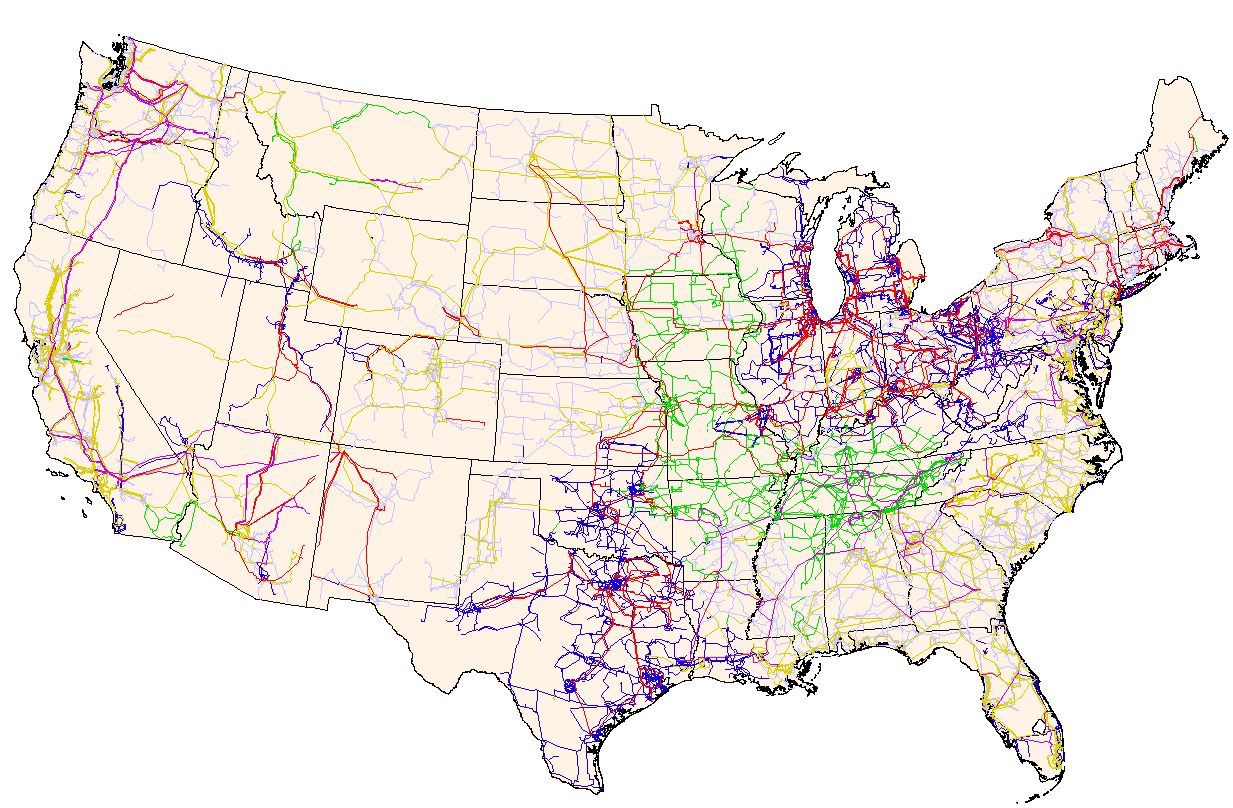 Figure 1. Complexity of electricity grids: the electric power transmission grid of the United States (source: FEMA and Wikipedia).
Power grids as graphs
Power grids are networks that include two main components: buses that represent important locations of the grid (e.g. generation points, load points, substations) and transmission (or distribution) lines that connect these buses.
It is pretty straightforward, therefore, to look at power grid networks as graphs: buses and transmission lines can be represented by nodes and edges of a corresponding graph.
There are two equivalent graph models that can be used to derive the basic power flow equations:
- directed graph representation (left panel of Figure 2): \(\mathbb{G}_{D}(\mathcal{N}, \mathcal{E})\);
- undirected graph representation (right panel of Figure 2): \(\mathbb{G}_{U}(\mathcal{N}, \mathcal{E} \cup \mathcal{E}^{R})\),
where \(\mathcal{N}\), \(\mathcal{E} \subseteq \mathcal{N} \times \mathcal{N}\) and \(\mathcal{E}^{R} \subseteq \mathcal{N} \times \mathcal{N}\) denote the set of nodes (buses), and the forward and reverse orientations of directed edges (branches) of the graph, respectively.
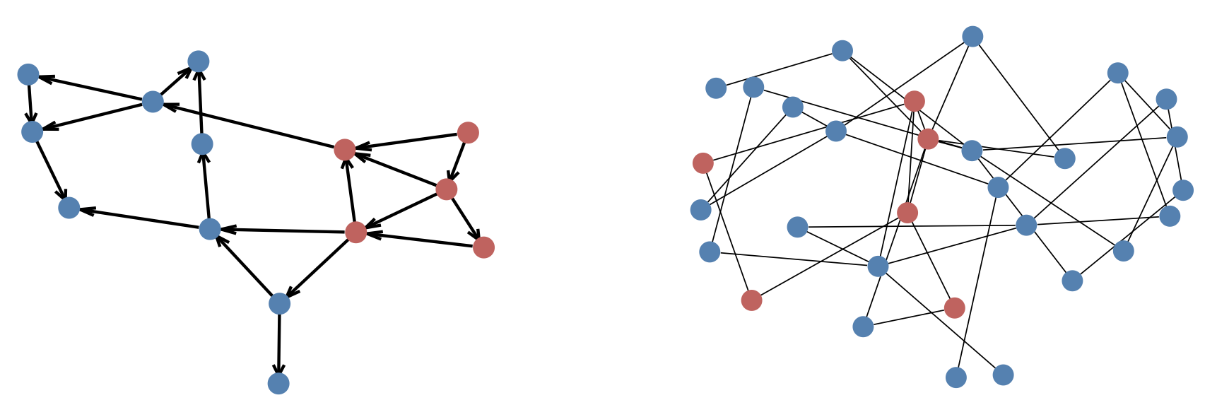 Figure 2. Directed graph representation of synthetic grid 14-ieee (left) and undirected graph representation of synthetic grid 30-ieee (right). Red and blue circles denote generator and load buses, respectively.
Complex power in AC circuits
Power can be transmitted more efficiently at high voltages as high voltage (or equivalently, low current) reduces the loss of power due to its dissipation on transmission lines.
Power grids generally use alternating current (AC) since the AC voltage can be altered (from high to low) easily via transformers.
Therefore, we start with some notation and definitions for AC circuits.
The most important characteristics of AC circuits is that, unlike in direct current (DC) circuits, the currents and voltages are not constant in time: both their magnitude and direction vary periodically.
Because of several technical reasons (like low losses and disturbances), power generators use sinusoidal alternating quantities that can be straightforwardly modeled by complex numbers.
We will consistently use capital and small letters to denote complex and real-valued quantities, respectively.
For instance, let us consider two buses, \(i, j \in \mathcal{N}\), that are directly connected by a transmission line \((i, j) \in \mathcal{E}\).
The complex power flowing from bus \(i\) to bus \(j\) is denoted by \(S_{ij}\) and it can be decomposed into its active (\(p_{ij}\)) and reactive (\(q_{ij}\)) components:
\[\begin{equation}
S_{ij} = p_{ij} + \mathrm{j}q_{ij},
\end{equation}\]
where \(\mathrm{j} = \sqrt{-1}\).
The complex power flow can be expressed as the product of the complex voltage at bus \(i\), \(V_{i}\) and the complex conjugate of the current flowing between the buses, \(I_{ij}^{*}\):
\[\begin{equation}
S_{ij} = V_{i}I_{ij}^{*},
\label{power_flow}
\end{equation}\]
It is well known that transmission lines have power losses due to their resistance (\(r_{ij}\)), which is a measure of the opposition to the flow of the current.
For AC-circuits, a dynamic effect caused by the line reactance (\(x_{ij}\)) also plays a role.
Unlike resistance, reactance does not cause any loss of power but has a delayed effect by storing and later returning power to the circuit.
The effect of resistance and reactance together can be represented by a single complex quantity, the impedance: \(Z_{ij} = r_{ij} + \mathrm{j}x_{ij}\).
Another useful complex quantity is the admittance, which is the reciprocal of the impedance: \(Y_{ij} = \frac{1}{Z_{ij}}\).
Similarly to the impedance, the admittance can be also decomposed into its real, conductance (\(g_{ij}\)), and imaginary, susceptance (\(b_{ij}\)), components: \(Y_{ij} = g_{ij} + \mathrm{j}b_{ij}\).
Therefore, the current can be written as a function of the line voltage drop and the admittance between the two buses, which is an alternative form of Ohm’s law:
\[\begin{equation}
I_{ij} = Y_{ij}(V_{i} - V_{j}).
\end{equation}\]
Replacing the above expression for the current in the power flow equation (eq. \(\eqref{power_flow}\)), we get
\[\begin{equation}
S_{ij} = Y_{ij}^{*}V_{i}V_{i}^{*} - Y_{ij}^{*}V_{i}V_{j}^{*} = Y_{ij}^{*} \left( |V_{i}|^{2} - V_{i}V_{j}^{*} \right).
\end{equation}\]
The above power flow equation can be expressed by using the polar form of voltage, i.e. \(V_{i} = v_{i}e^{\mathrm{j} \delta_{i}} = v_{i}(\cos\delta_{i} + \mathrm{j}\sin\delta_{i})\) (where \(v_{i}\) and \(\delta_{i}\) are the voltage magnitude and angle of bus \(i\), respectively), and the admittance components:
\[\begin{equation}
S_{ij} = \left(g_{ij} - \mathrm{j}b_{ij}\right) \left(v_{i}^{2} - v_{i}v_{j}\left(\cos\delta_{ij} + \mathrm{j}\sin\delta_{ij}\right)\right),
\end{equation}\]
where for brevity we introduced the voltage angle difference \(\delta_{ij} = \delta_{i} - \delta_{j}\).
Similarly, using a simple algebraic identity of \(g_{ij} - \mathrm{j}b_{ij} = \frac{g_{ij}^{2} + b_{ij}^{2}}{g_{ij} + \mathrm{j}b_{ij}} = \frac{|Y_{ij}|^{2}}{Y_{ij}} = \frac{Z_{ij}}{|Z_{ij}|^{2}} = \frac{r_{ij} + \mathrm{j}x_{ij}}{r_{ij}^{2} + x_{ij}^{2}}\), the impedance components-based expression has the following form:
\[\begin{equation}
S_{ij} = \frac{r_{ij} + \mathrm{j}x_{ij}}{r_{ij}^{2} + x_{ij}^{2}} \left( v_{i}^{2} - v_{i}v_{j}\left(\cos\delta_{ij} + \mathrm{j}\sin\delta_{ij}\right)\right).
\end{equation}\]
Finally, the corresponding real equations can be written as
\[\begin{equation}
\left\{
\begin{aligned}
p_{ij} & = g_{ij} \left( v_{i}^{2} - v_{i} v_{j} \cos\delta_{ij} \right) - b_{ij} \left( v_{i} v_{j} \sin\delta_{ij} \right) \\
q_{ij} & = b_{ij} \left( -v_{i}^{2} + v_{i} v_{j} \cos\delta_{ij} \right) - g_{ij} \left( v_{i} v_{j} \sin\delta_{ij} \right), \\
\end{aligned}
\right.
\label{power_flow_y}
\end{equation}\]
and
\[\begin{equation}
\left\{
\begin{aligned}
p_{ij} & = \frac{1}{r_{ij}^{2} + x_{ij}^{2}} \left[ r_{ij} \left( v_{i}^{2} - v_{i} v_{j} \cos\delta_{ij} \right) + x_{ij} \left( v_{i} v_{j} \sin\delta_{ij} \right) \right] \\
q_{ij} & = \frac{1}{r_{ij}^{2} + x_{ij}^{2}} \left[ x_{ij} \left( v_{i}^{2} - v_{i} v_{j} \cos\delta_{ij} \right) + r_{ij} \left( v_{i} v_{j} \sin\delta_{ij} \right) \right]. \\
\end{aligned}
\right.
\label{power_flow_z}
\end{equation}\]
Power flow models
In the previous section we presented the power flow between two connected buses and established a relationship between complex power flow and complex voltages.
In power flow problems, the entire power grid is considered and the task is to calculate certain quantities based on some other specified ones.
There are two equivalent power flow models depending on the graph model used: the bus injection model (based on the undirected graph representation) and the branch flow model (based on the directed graph representation).
First, we introduce the basic formulations.
Then, we show the most widely used technique to solve power flow problems.
Finally, we extend the basic equations and derive more sophisticated models including additional components for real power grids.
Bus injection model
The bus injection model (BIM) uses the undirected graph model of the power grid, \(\mathbb{G}_{U}\).
For each bus \(i\), we denote by \(\mathcal{N}_{i} \subset \mathcal{N}\) the set of buses directly connected to bus \(i\).
Also, for each bus we introduce the following quantities (Figure 3):
- \(S_{i}^{\mathrm{gen}}\): generated power flowing into bus \(i\).
- \(S_{i}^{\mathrm{load}}\): demand power or load flowing out of the bus \(i\).
- \(S_{i}\): net power injection at bus \(i\), i.e. \(S_{i} = S_{i}^{\mathrm{gen}} - S_{i}^{\mathrm{load}}\).
- \(S_{i}^{\mathrm{trans}}\): transmitted power flowing between bus \(i\) and its adjacent buses.
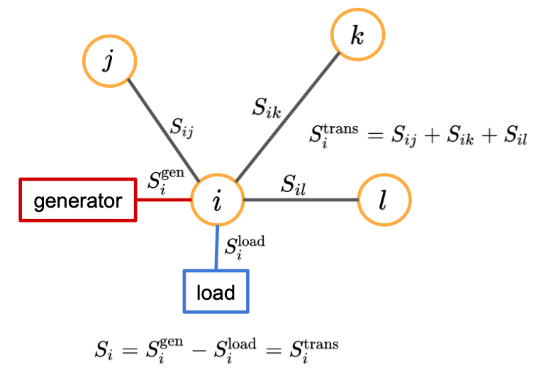 Figure 3. Power balance and quantities of a bus connected to three adjacent buses and including a single generator and a single load.
Tellegen’s theorem establishes a simple relationship between these power quantities:
\[\begin{equation}
S_{i} = S_{i}^{\mathrm{gen}} - S_{i}^{\mathrm{load}} = S_{i}^{\mathrm{trans}} \ \ \ \ \forall i \in \mathcal{N}.
\label{power_balance}
\end{equation}\]
Eq. \(\eqref{power_balance}\) expresses the law of conservation of power (energy): the power injected (\(S_{i}^{\mathrm{gen}}\)) to bus \(i\) must be equal to the power going out from the bus, i.e. the sum of the withdrawn (\(S_{i}^{\mathrm{load}}\)) and transmitted power (\(S_{i}^{\mathrm{trans}}\)).
In the most basic model, a bus can represent either a generator (i.e. \(S_{i} = S_{i}^{\mathrm{gen}}\)) or a load (i.e. \(S_{i} = -S_{i}^{\mathrm{load}}\)).
For a given bus, the transmitted power can be obtained simply as a sum of the powers flowing in to and out from the bus, \(S_{i}^{\mathrm{trans}} = \sum \limits_{j \in \mathcal{N}_{i}} S_{ij}\).
Therefore, the basic BIM has the following concise form:
\[\begin{equation}
S_{i} = \sum \limits_{j \in \mathcal{N}_{i}} Y_{ij}^{*} \left( |V_{i}|^{2} - V_{i}V_{j}^{*} \right) \ \ \ \ \forall i \in \mathcal{N} .
\label{bim_basic_concise}
\end{equation}\]
Branch flow model
We briefly describe an alternative formulation of the power flow problem, the branch flow model (BFM).
The BFM is based on the directed graph representation of the grid network, \(\mathbb{G}_{D}\), and directly models branch flows and currents.
Let us fix an arbitrary orientation of \(\mathbb{G}_{D}\) and let \((i, j) \in \mathcal{E}\) denote an edge pointing from bus \(i\) to bus \(j\).
Then, the BFM is defined by the following set of complex equations:
\[\begin{equation}
\left\{
\begin{aligned}
S_{i} & = \sum \limits_{(i, j) \in \mathcal{E}_{D}} S_{ij} - \sum \limits_{(k, i) \in \mathcal{E}} \left( S_{ki} - Z_{ki} |I_{ki}|^{2} \right) & \forall i \in \mathcal{N}, \\
I_{ij} & = Y_{ij} \left( V_{i} - V_{j} \right) & \forall (i, j) \in \mathcal{E}, \\
S_{ij} & = V_{i}I_{ij}^{*} & \forall (i, j) \in \mathcal{E}, \\
\end{aligned}
\right.
\label{bfm_basic_concise}
\end{equation}\]
where the first, second and third sets of equations correspond to the power balance, Ohm’s law, and branch power definition, respectively.
The power flow problem
The power flow problem is to find a unique solution of a power system (given certain input variables) and, therefore, it is central to power grid analysis.
First, let us consider the BIM equations (eq. \(\eqref{bim_basic_concise}\)) that define a complex non-linear system with \(N = |\mathcal{N}|\) complex equations, and \(2N\) complex variables, \(\left\{S_{i}, V_{i}\right\}_{i=1}^{N}\).
Equivalently, either using the admittance (eq. \(\eqref{power_flow_y}\))
or the impedance (eq. \(\eqref{power_flow_z}\))
components we can construct \(2N\) real equations with \(4N\) real variables: \(\left\{p_{i}, q_{i}, v_{i}, \delta_{i}\right\}_{i=1}^{N}\), where \(S_{i} = p_{i} + \mathrm{j}q_{i}\).
The power flow problem is the following: for each bus we specify two of the four real variables and then using the \(2N\) equations we derive the remaining variables.
Depending on which variables are specified there are three basic types of buses:
- Slack (or \(V\delta\) bus) is usually a reference bus, where the voltage angle and magnitude are specified. Also, slack buses are used to make up any generation and demand mismatch caused by line losses. The voltage angle is usually set to 0, while the magnitude to 1.0 per unit.
- Load (or \(PQ\) bus) is the most common bus type, where only demand but no power generation takes place. For such buses the active and reactive powers are specified.
- Generator (or \(PV\) bus) specifies the active power and voltage magnitude variables.
Table 1. Basic bus types in power flow problem.
| Bus type |
Code |
Specified variables |
| Slack |
\(V\delta\) |
\(v_{i}\), \(\delta_{i}\) |
| Load |
\(PQ\) |
\(p_{i}\), \(q_{i}\) |
| Generator |
\(PV\) |
\(p_{i}\), \(v_{i}\) |
Further, let \(E = |\mathcal{E}|\) denote the number of directed edges.
The BFM formulation (eq. \(\eqref{bfm_basic_concise}\)) includes \(N + 2E\) complex equations with \(2N + 2E\) complex variables: \(\left\{ S_{i}, V_{i} \right\}_{i \in \mathcal{N}} \cup \left\{ S_{ij}, I_{ij} \right\}_{(i, j) \in \mathcal{E}}\) or equivalently, \(2N + 4E\) real equations with \(4N + 4E\) real variables.
BIM vs BFM
The BIM and the BFM are equivalent formulations, i.e. they define the same physical problem and provide the same solution.
Although the formulations are equivalent, in practice we might prefer one model over the other.
Depending on the actual problem and the structure of the system, it might be easier to obtain results and derive an exact solution or an approximate relaxation from one formulation than from the other one.
Table 2. Comparison of basic BIM and BFM formulations: complex variables, number of complex variables and equations. Corresponding real variables, their numbers as well as the number of real equations are also shown in parentheses.
| Formulation |
Variables |
Number of variables |
Number of equations |
| BIM |
\(V_{i} \ (v_{i}, \delta_{i})\)
\(S_{i} \ (p_{i}, q_{i})\) |
\(2N\)
\((4N)\) |
\(N\)
\((2N)\) |
| BFM |
\(V_{i} \ (v_{i}, \delta_{i})\)
\(S_{i} \ (p_{i}, q_{i})\)
\(I_{ij} \ (i_{ij}, \gamma_{ij})\)
\(S_{ij} \ (p_{ij}, q_{ij})\) |
\(2N + 2E\)
\((4N + 4E)\) |
\(N + 2E\)
\((2N + 4E)\) |
Solving the power flow problem
Power flow problems (formulated as either a BIM or a BFM) define a non-linear system of equations.
There are multiple approaches to solve power flow systems but the most widely used technique is the Newton–Raphson method.
Below we demonstrate how it can be applied to the BIM formulation.
First, we rearrange eq. \(\eqref{bim_basic_concise}\):
\[\begin{equation}
F_{i} = S_{i} - \sum \limits_{j \in \mathcal{N}_{i}} Y_{ij}^{*} \left( |V_{i}|^{2} - V_{i}V_{j}^{*} \right) = 0 \ \ \ \ \forall i \in \mathcal{N}.
\end{equation}\]
The above set of equations can be expressed simply as \(F(X) = 0\), where \(X\) denotes the \(N\) complex or more conveniently, the \(2N\) real unknown variables and \(F\) represents the \(N\) complex or \(2N\) real equations.
In the Newton—Raphson method the solution is sought in an iterative fashion, until a certain threshold of convergence is satisfied.
In the \((n+1)\)th iteration we obtain:
\[\begin{equation}
X_{n+1} = X_{n} - J_{F}(X_{n})^{-1} F(X_{n}),
\end{equation}\]
where \(J_{F}\) is the Jacobian matrix with \(\left[J_{F}\right]_{ij} = \frac{\partial F_{i}}{\partial X_{j}}\) elements.
We also note that, instead of computing the inverse of the Jacobian matrix, a numerically more stable approach is to solve first a linear system of \(J_{F}(X_{n}) \Delta X_{n} = -F(X_{n})\) and then obtain \(X_{n+1} = X_{n} + \Delta X_{n}\).
Since Newton—Raphson method requires only the computation of first derivatives of the \(F_{i}\) functions with respect to the variables, this technique is in general very efficient even for large, real-size grids.
Towards more realistic power flow models
In the previous sections we introduced the main concepts needed to understand and solve the power flow problem.
However, the derived models were rather basic ones, and real systems require more reasonable approaches.
Below we will construct more sophisticated models by extending the basic equations considering the following:
- multiple generators and loads included in buses;
- shunt elements connected to buses;
- modeling transformers and phase shifters;
- modeling asymmetric line charging.
We note that actual power grids can include additional elements besides the ones we discuss.
Improving the bus model
We start with the generated (\(S_{i}^{\mathrm{gen}}\)) and load (\(S_{i}^{\mathrm{load}}\)) powers in the power balance equations, i.e. \(S_{i} = S_{i}^{\mathrm{gen}} - S_{i}^{\mathrm{load}} = S_{i}^{\mathrm{trans}}\) for each bus \(i\).
Electric grid buses can actually include multiple generators and loads together.
In order to take this structure into account we introduce \(\mathcal{G}_{i}\) and \(\mathcal{L}_{i}\), denoting the set of generators and the set of loads at bus \(i\), respectively.
Also, \(\mathcal{G} = \bigcup \limits_{i \in \mathcal{N}} \mathcal{G}_{i}\) and \(\mathcal{L} = \bigcup \limits_{i \in \mathcal{N}} \mathcal{L}_{i}\) indicate the sets of all generators and loads, respectively.
Then we can write the following complex-valued expressions:
\[\begin{equation}
S_{i}^{\mathrm{gen}} = \sum \limits_{g \in \mathcal{G}_{i}} S_{g}^{G} \ \ \ \ \forall i \in \mathcal{N},
\end{equation}\]
\[\begin{equation}
S_{i}^{\mathrm{load}} = \sum \limits_{l \in \mathcal{L}_{i}} S_{l}^{L} \ \ \ \ \forall i \in \mathcal{N},
\end{equation}\]
where \(\left\{S_{g}^{G}\right\}_{g \in \mathcal{G}}\) and \(\left\{S_{l}^{L}\right\}_{l \in \mathcal{L}}\) are the complex powers of generator dispatches and load consumptions, respectively.
It is easy to see from the equations above that having multiple generators and loads per bus increases the total number of variables, while the number of equations does not change.
If the system includes \(N = \lvert \mathcal{N} \rvert\) buses, \(G = \lvert \mathcal{G} \rvert\) generators and \(L = \lvert \mathcal{L} \rvert\) loads, then the total number of complex variables changes to \(N + G + L\) and \(N + G + L + 2E\) for BIM and BFM, respectively.
Buses can also include shunt elements that are used to model connected capacitors and inductors.
They are represented by individual admittances resulting in additional power flowing out of the bus:
\[\begin{equation}
S_{i} = S_{i}^{\mathrm{gen}} - S_{i}^{\mathrm{load}} - S_{i}^{\mathrm{shunt}} = \sum \limits_{g \in \mathcal{G}_{i}} S_{g}^{G} - \sum \limits_{l \in \mathcal{L}_{i}} S_{l}^{L} - \sum \limits_{s \in \mathcal{S}_{i}} S_{s}^{S} \ \ \ \ \forall i \in \mathcal{N},
\end{equation}\]
where \(\mathcal{S}_{i}\) is the set of shunts attached to bus \(i\) and \(S^{S}_{s} = \left( Y_{s}^{S} \right)^{*} \lvert V_{i} \rvert^{2}\) with admittance \(Y_{s}^{S}\) of shunt \(s \in \mathcal{S}_{i}\).
Shunt elements do not introduce additional variables in the system.
Improving the branch model
In real power grids, branches can be transmission lines, transformers, or phase shifters.
Transformers are used to control voltages, active and, sometimes, reactive power flows.
In this section we take the transformer and line charging also into account by a general branch model (Figure 4).
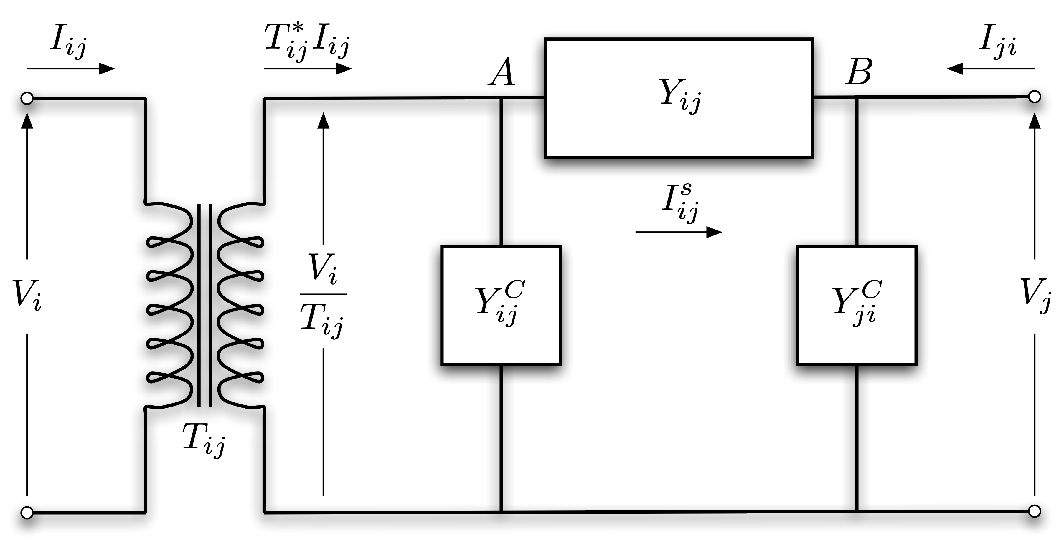 Figure 4. General branch model including transformers and \(\pi\)-section model (source: MATPOWER manual).
Transformers (and also phase shifters) are represented by the complex tap ratio \(T_{ij}\), or equivalently, by its magnitude \(t_{ij}\) and phase angle \(\theta_{ij}\).
Also, line charging is usually modeled by the \(\pi\) transmission line (or \(\pi\)-section) model, which places shunt admittances at the two ends of the transmission line, beside its series admittance.
We will treat the shunt admittances in a fairly general way, i.e. \(Y_{ij}^{C}\) and \(Y_{ji}^{C}\) are not necessarily equal but we also note that a widely adopted practice is to assume equal values and consider their susceptance component only.
Since this model is not symmetric anymore, for consistency we introduce the following convention: we select the orientation of each branch \((i, j) \in \mathcal{E}\) that matches the structure presented in Figure 4.
In order to derive the corresponding power flow equations of this model (for both directions due to the asymmetric arrangement), we first look for expressions of the current \(I_{ij}\) and \(I_{ji}\).
The transformer alters the input voltage \(V_{i}\) and current \(I_{ij}\).
Using the complex tap ratio the output voltage and current are \(\frac{V_{i}}{T_{ij}}\) and \(T_{ij}^{*}I_{ij}\), respectively.
Let \(I_{ij}^{s}\) denote the series current flowing between point \(A\) and \(B\) in Figure 4.
Based on Kirchhoff’s current law the net current flowing into node \(A\) is equal to the net current flowing out from it, i.e. \(T_{ij}^{*} I_{ij} = I_{ij}^{s} + Y_{ij}^{C} \frac{V_{i}}{T_{ij}}\).
Rearranging this expression for \(I_{ij}\) we get:
\[\begin{equation}
I_{ij} = \frac{I_{ij}^{s}}{T_{ij}^{*}} + Y_{ij}^{C} \frac{V_{i}}{\lvert T_{ij} \rvert^{2}} \quad \forall (i, j) \in \mathcal{E}.
\end{equation}\]
Similarly, applying Kirchhoff’s current law for node \(B\) we can obtain \(I_{ji}\):
\[\begin{equation}
I_{ji} = -I_{ij}^{s} + Y_{ji}^{C} V_{j} \quad \forall (j, i) \in \mathcal{E}^{R}.
\end{equation}\]
Finally, using again Ohm’s law, the series current has the following simple expression: \(I_{ij}^{s} = Y_{ij} \left( \frac{V_{i}}{T_{ij}} - V_{j} \right)\).
Now we can easily obtain the corresponding power flows:
\[\begin{equation}
\begin{aligned}
S_{ij} & = V_{i}I_{ij}^{*} = V_{i} \left( \frac{I_{ij}^{s}}{T_{ij}^{*}} + Y_{ij}^{C} \frac{V_{i}}{\lvert T_{ij} \rvert^{2}}\right)^{*} & \\
& = Y_{ij}^{*} \left( \frac{\lvert V_{i} \rvert^{2}}{\lvert T_{ij} \rvert^{2}} - \frac{V_{i} V_{j}^{*}}{T_{ij}} \right) + \left( Y_{ij}^{C} \right)^{*} \frac{\lvert V_{i} \rvert^{2}}{\lvert T_{ij} \rvert^{2}} \ \ \ \ & \forall (i, j) \in \mathcal{E} \\
S_{ji} & = V_{j}I_{ji}^{*} = V_{j} \left( -I_{ij}^{s} + Y_{ji}^{C}V_{j} \right)^{*} & \\
& = Y_{ij}^{*} \left( \lvert V_{j} \rvert^{2} - \frac{V_{j}V_{i}^{*}}{T_{ij}^{*}} \right) + \left( Y_{ji}^{C} \right)^{*} \lvert V_{j} \rvert^{2} \ \ \ \ & \forall (j, i) \in \mathcal{E}^{R} \\
\end{aligned}
\end{equation}\]
Improved BIM and BFM models
Putting everything together from the previous sections we present the improved BIM and BFM models:
BIM:
\[\begin{equation}
\begin{aligned}
\sum \limits_{g \in \mathcal{G}_{i}} S_{g}^{G} - \sum \limits_{l \in \mathcal{L}_{i}} S_{l}^{L} - \sum \limits_{s \in \mathcal{S}_{i}} \left( Y_{s}^{S} \right)^{*} \lvert V_{i} \rvert^{2} = \sum \limits_{(i, j) \in \mathcal{E}} Y_{ij}^{*} \left( \frac{\lvert V_{i} \rvert^{2}}{\lvert T_{ij} \rvert^{2}} - \frac{V_{i} V_{j}^{*}}{T_{ij}} \right) + \left( Y_{ij}^{C} \right)^{*} \frac{\lvert V_{i} \rvert^{2}}{\lvert T_{ij} \rvert^{2}} \\
+ \sum \limits_{(k, i) \in \mathcal{E}^{R}} Y_{ik}^{*} \left( \lvert V_{k} \rvert^{2} - \frac{V_{k}V_{i}^{*}}{T_{ik}^{*}} \right) + \left( Y_{ki}^{C} \right)^{*} \lvert V_{k} \rvert^{2} \ \ \ \ \forall i \in \mathcal{N}, \\
\end{aligned}
\label{bim_concise}
\end{equation}\]
where, on the left-hand side, the net power at bus \(i\) is computed from the power injection of multiple generators and power withdrawals of multiple loads and shunt elements, while, on the right-hand side, the transmitted power is a sum of the outgoing (first term) and incoming (second term) power flows to and from the corresponding adjacent buses.
BFM:
\[\begin{equation}
\begin{aligned}
& \sum \limits_{g \in \mathcal{G}_{i}} S_{g}^{G} - \sum \limits_{l \in \mathcal{L}_{i}} S_{l}^{L} - \sum \limits_{s \in \mathcal{S}_{i}} \left( Y_{s}^{S} \right)^{*} \lvert V_{i} \rvert^{2} = \sum \limits_{(i, j) \in \mathcal{E}} S_{ij} + \sum \limits_{(k, i) \in \mathcal{E}^{R}} S_{ki} & \forall i \in \mathcal{N} \\
& I_{ij}^{s} = Y_{ij} \left( \frac{V_{i}}{T_{ij}} - V_{j} \right) & \forall (i, j) \in \mathcal{E} \\
& S_{ij} = V_{i} \left( \frac{I_{ij}^{s}}{T_{ij}^{*}} + Y_{ij}^{C} \frac{V_{i}}{\lvert T_{ij} \rvert^{2}}\right)^{*} & \forall (i, j) \in \mathcal{E} \\
& S_{ji} = V_{j} \left( -I_{ij}^{s} + Y_{ji}^{C}V_{j} \right)^{*} & \forall (j, i) \in \mathcal{E}^{R} \\
\end{aligned}
\label{bfm_concise}
\end{equation}\]
As before, BFM is an equivalent formulation to BIM (first set of equations), with the only difference being that BFM treats the series currents (second set of equations) and power flows (third and fourth sets of equations) as explicit variables.
Table 3. Comparison of improved BIM and BFM formulations: complex variables, number of complex variables and equations. Corresponding real variables, their numbers as well as the number of real equations are also shown in parentheses.
| Formulation |
Variables |
Number of variables |
Number of equations |
| BIM |
\(V_{i} \ (v_{i}, \delta_{i})\)
\(S_{g}^{G} \ (p_{g}^{G}, q_{g}^{G})\)
\(S_{l}^{L} \ (p_{l}^{L}, q_{l}^{L})\) |
\(N + G + L\)
\((2N + 2G + 2L)\) |
\(N\)
\((2N)\) |
| BFM |
\(V_{i} \ (v_{i}, \delta_{i})\)
\(S_{g}^{G} \ (p_{g}^{G}, q_{g}^{G})\)
\(S_{l}^{L} \ (p_{l}^{L}, q_{l}^{L})\)
\(I_{ij}^{s} \ (i_{ij}^{s}, \gamma_{ij}^{s})\)
\(S_{ij} \ (p_{ij}, q_{ij})\)
\(S_{ji} \ (p_{ji}, q_{ji})\) |
\(N + G + L + 3E\)
\((2N + 2G + 2L + 6E)\) |
\(N + 3E\)
\((2N + 6E)\) |
Conclusions
In this blog post, we introduced the main concepts of the power flow problem and derived the power flow equations for a basic and a more realistic model using two equivalent formulations.
We also showed that the resulting mathematical problems are non-linear systems that can be solved by the Newton—Raphson method.
Solving power flow problems is essential for the analysis of power grids.
Based on a set of specified variables, the power flow solution provides the unknown ones.
Consider a power grid with \(N\) buses, \(G\) generators and \(L\) loads, and let us specify only the active and reactive powers of the loads, which means \(2L\) number of known real-valued variables.
Whichever formulation we use, this system is underdetermined and we would need to specify \(2G\) additional variables (Table 3.) to obtain a unique solution.
However, generators have distinct power supply capacities and cost curves, and we can ask an interesting question: among the many physically possible specifications of the generator variables which is the one that would minimize the total economic cost?
This question leads to the mathematical model of economic dispatch, which is one of the most widely used optimal power flow problems.
Optimal power flow problems are constrained optimization problems that are based on the power flow equations with additional physical constraints and an objective function.
In our next post, we will discuss the main types and components of optimal power flow, and show how exact and approximate solutions can be obtained for these significantly more challenging problems.
06 Nov 2020
Author: Sam Morrison
Over the last two years, our Julia codebase has grown in size and complexity, and is now the centerpiece of both our operations and research.
This implies that we need to routinely replace parts of the system like puzzle pieces, and carefully test if the results lead to improvements along various dimensions of performance.
However, those pieces are not designed to work in isolation, and thus cannot be tested in a vacuum.
They also tend to be quite large and complex, and therefore often need to be independent packages, which need to “fit” together in precise ways determined by the rest of the system.
This is where interfaces come in handy: they are tools for isolating and precisely testing specific pieces of a large system.
In order to have the option of reusing an interface without pulling in a lot of extra code, we avoid embedding the interface into any package using it, allowing it to exist in a package on its own.
This approach also makes it easier to keep track of the changes to the interface, when these are not tied to unrelated changes in other packages.
This results in a set of very slim interface packages that define what functional pieces need to be filled in and how they should fit.
Interface Packages
For our purposes, an interface package is any Julia package that contains an abstract type with no concrete implementation—a sort of IOU in code.
Most functions defined for the type are either un-implemented or are based on other, un-implemented functions.
Despite having very little code, the docstrings form a sort of contract laying out what methods a concrete implementation should have and what they should do in order for the implementation to be considered valid.
A package implementing the interface but missing methods or using different function signatures from interface package can be said to break the contract.
As long as the contract between the concrete and abstract interface remains unbroken, a package using the interface should be able to swap out any concrete implementation for any other and still run as expected provided the user package is using the interface as documented.
In order to improve the modularity of the code, they are separated from the code that uses the abstract type.
This results in interface packages essentially looking like design documents.
For example, below we sketch an interface package for a database.
module AbstractDB

"""
    AbstractDB

A simple API for read only access to a database.
"""
abstract type AbstractDB end

"""
    AbstractResponse

Query data needed for fetch.
"""
abstract type AbstractResponse end

"""
    query(
        db::AbstractDB,
        table::String,
        features::Vector{Feature}
    ) -> AbstractResponse

Submit an appropriate query to `table` in `db` asking for results matching
`features`.
"""
function query end


"""
    fetch(
        db::AbstractDB,
        response::Union{Response,Vector{Response}}
    ) -> DataFrame

Retrieve the results from `response` and parses them into a `DataFrame`.
"""
function fetch end

"""
    easy_query(
        db::AbstractDB,
        table::String,
        features::Vector{Feature}
    ) -> DataFrame

Submit  and fetches a query to `table` in `db` asking for results matching
`features`.
"""
function easy_query(db::AbstractDB, table::String, features::Vector{Feature})
    return fetch(db, query(db, table, features))
end

end
For our purposes, we will assume a Feature type exists and corresponds to a column in a database table with some criteria for selecting rows.
We will also assume that filtering a DataFrame by some Features works, but is too inefficient to be used in practice.
A problem with interface packages
While simple to write, interface packages can fall victim to a common failure.
Since interface packages provide little more than function names and docstrings, it’s easy for the packages around them to “go rogue”, changing the function signatures for the interface as they see fit without updating the actual interface package.
This ends up creating a secret, undocumented interface known only to the implemented types and whichever packages manage to use them.
For example, let’s say a concrete subtype of our AbstractDB database example above changes to let a user define a fancy transform to join up results during fetch in a new version.
# RogueDB.jl
fetch(db::RogueDB, response::Vector{Response}, fancy_transform::Callable)
easy_query(
    db::RogueDB,
    table::String,
    features::Vector{Feature},
    fancy_transform=donothing()
)
The fancy_transform has a fallback and does not break the contract the interface sets out, but it can cause problems if other packages only refer back to RogueDB.
If another package X claims to use an AbstractDB but makes use of the fancy_transform in both functions and doesn’t fall back to the documented version of fetch, it now can’t switch to another AbstractDB.
This goes unnoticed, as X is only tested against RogueDB.
Say we now want to hook up another DB to X so we make the fetch function when NewDB is created.
# NewDB.jl
fetch(db::NewDB, response::Vector{Response}, fancy_transform::Callable)
The above fetch does break the contract with the interface package, but X has been used for several months and nobody questions the API, so fetch without the fancy_transform is not implemented.
X uses the default easy_query with NewDB, which does not include the fancy_transform argument.
Calling easy_query will cause a MethodError, but X only calls that function in an untested (or mocked) special case and the bug goes unseen.
Further suppose that AbstractDB has been at v0.1 for 2 years and still has the original definition of fetch.
There are several other DB packages being used in other packages that use the documented fetch, but nobody has noticed they are different.
Now the interface package doesn’t serve its purpose, as other packages using the interface as documented will fail to run the rogue implementations.
New implementations will have to guess at the secret interface set up by the rogue packages in order to fit into the existing ecosystem.
The version of the interface being used is dependent upon multiple packages, potentially causing chaos!
Test Utils
Having a robust set of test utilities gives an interface package enough muscle to enforce the contract it sets out.
A good test utility for an interface package contains two key components:
- A test fake: a simplified implementation of the type for user packages to play with.
- A test suite codifying a minimum set of constraints an implementation must obey to be considered legitimate.
The Test Suite
How?
The test suite is a function or set of functions that work as a validation test for a concrete implementation of a type.
It should codify the expectations of the abstract type (e.g., function signatures, return types) as precisely as possible.
The tests should check that a new implementation does not break the contract that an abstract type sets out.
The test suite should simply test that the interface for the type works as expected.
It does not replace unit tests for the correctness of output or any special-cased behaviour, nor can it be expected to check any implementation details or corner cases.
The test suites should be run as part of the unit tests for any implementation of the type.
If the API changes, it should give instant feedback when the expectations of the abstract type are not met.
A minimal test suite for the database example might look like the following:
"""
    test_interface(db::AbstractDB, table::String, features::Vector{Feature})

Check if an `AbstractDB` follows the documented structure.
The arguments supplied to this function should be identical to those for a
successful `query`.
"""
function test_interface(db::AbstractDB, table::String, features::Vector{Feature})
    q = query(db, table, features)
    @test q isa AbstractResponse

    df = fetch(db, resp)
    @test df isa DataFrame

    @test filter(df, features) == df

    # Check easy_query gives the same results as long form
    @test easy_query(db, table, features) == df

    resp2 = fetch(db, [resp, resp])
    @test resp2 isa AbstractResponse
    @test fetch(db, resp) isa DataFrame
end
Why?
The test suite puts the power to define the API back into the hands of the interface package.
A package using these tests can be trusted to have defined the functions we need in the form that we expect, so long as the tests pass.
When the interface package changes, the failing tests will serve as a sign to update all related packages to stay consistent with the interface.
The test suite is also handy for creating new implementations.
The test suite is ready-made to be used in test-driven development and helps clear up any ambiguities that might exist in the docstrings.
The Test Fake
How?
Test fakes are a kind of test double.
They have a working implementation but take some shortcuts, which makes them suitable only for testing functionality.
Ideally, a test fake should:
- Be easy to construct.
- Only enact the minimum expectations of the API for the abstract type.
- Give easily verifiable outputs.
Test fakes should be used in tests for any package using the abstract type in order to avoid depending on any “real” version.
Below we show what a lazy implementation of a test fake for the database example might look like:
struct FakeDB <: AbstractDB
    data::Dict{String, DataFrame}
end

struct FakeResponse <: AbstractResponse
    fetched::DataFrame
end

FakeDB(data_dir::Path) = FakeDB(populate_data(data_dir))

function query(db::FakeDB, table::String, features::Vector{Feature})
    data = db[table]
    return FakeResponse(filter(data, features))
end

fetch(::FakeDB, r::FakeResponse) = r.fetched
fetch(::FakeDB, rs::Vector{FakeResponse}) = join(fetch.(rs)…)
To make sure things are consistent, the test_interface function from the section above should be run on FakeDB as part of the tests for AbstractDB.
Why?
Because the test fake is included as part of the interface package, it can be trusted to enact the interface as advertised.
Any code using the fake can be expected to work with any legitimate implementation of the interface that is already passing tests with the test suite.
Since they are minimal examples, they are unlikely to stray from the interface-defined API by adding extra functions that user packages may mistakenly begin to depend on.
Test fakes also help to keep user packages in line with the interface package versions.
When the interface changes, the fakes change and the user code can be fixed to stay consistent with the interface package.
Test fakes can be especially useful shortcuts if a “real” implementation would be awkward to construct or would rely on network access, as they are usually locally-hosted, simplified examples.
Conclusion
Robust testing for interface packages helps reduce confusion about how abstract types work.
People who are new to the interface can look at the test suite to know how information will flow and can use the included tests as a sanity check while making changes to a concrete implementation.
The test fakes give users a toy example to play with and a minimum set of requirements for what a “real” implementation must do.
The test utilities also create a clear separation of concerns between the packages implementing the code and the packages using the code.
Combined with the docstrings, the test suite should provide implementer packages with all the structure the code needs.
Likewise, the test fakes should let user packages test their code without having to depend on a possibly incorrect implementer package.
Neither side should have to look at the details of the other to know how to use the interface itself.
Lastly, forcing both user and implementer packages to test against the interface package guarantees that the version number of the interface package dictates the version of the interface API both can use.
If an interface adds or changes a function and the implementer hasn’t added it, the test suite will fail.
If an interface removes or changes a function and the user package is testing against the test fake, the tests will fail.
If two packages are added using conflicting versions of the API, assuming both packages have bounded the interface package, we get a useful version conflict rather than unexpected behaviour.
Adding interface testing helps interface packages do their job, helping users be sure that when they run their code, a piece will fit where it should without the whole puzzle falling apart.
12 Aug 2020
Author: Andrew Rosemberg, Chris Davis, Glenn Moynihan, Matt Brzezinski, and Will Tebbutt
We at Invenia are heavy users of Julia, and are proud to once again have been a part of this year’s JuliaCon. This was the first year the conference was fully online, with about 10,000 registrations and 26,000 people tuning in. Besides being sponsors of the conference, Invenia also had several team members attending, helping host sessions, and presenting some of their work.
This year we had five presentations: “Design documents are great, here’s why you should consider one”, by Matt Brzezinski; “ChainRules.jl”, by Frames Catherine White; “HydroPowerModels.jl: Impacts of Network Simplifications”, by Andrew Rosemberg; “Convolutional Conditional Neural Processes in Flux”, by Wessel Bruinsma; and “Fast Gaussian processes for time series”, by Will Tebbutt.
JuliaCon always brings some really exciting work, and this year it was no different. We are eager to share some of our highlights.
JuliaCon is not just about research
There were a lot of good talks and workshops at JuliaCon this year, but one which stood out was “Building microservices and applications in Julia”, by Jacob Quinn. This workshop was about creating a music album management microservice, and provided useful information for both beginners and more experienced users. Jacob explained how to define the architectural layers, solving common problems such as authentication and caching, as well as deploying the service to Google Cloud Platform.
A very interesting aspect of the talk was that it exposed Julia users to the field of software engineering. JuliaCon usually has a heavy emphasis on academic and research-focused talks, so it was nice to see the growth of a less represented field within the community. There were a few other software engineering related talks, but having a hands-on practical approach is a great way to showcase a different approach to architecting code.
Among the other software engineering talks and posters, we can highlight “Reproducible environments with Singularity”, by Steffen Ridderbusch; the aforementioned “Design documents are great, here’s why you should consider one”, by Matt Brzezinski; “Dispatching Design Patterns”, by Aaron Christianson; and “Fantastic beasts and how to show them”, by Joris Kraak.
The conference kicked off with a brief and fun session on work related to Gaussian processes, including our own Will Tebbutt who talked about TemporalGPs.jl, which provides fast inference for certain types of GP models for time series, as well as Théo Galy-Fajou’s talk on KernelFunctions.jl. Although there was no explicit talk on the topic, there were productive discussions about the move towards a common set of abstractions provided by AbstractGPs.jl.
It was also great to see so many people at the Probabilistic Programming Bird of a Feather, and it feels like there is a proper community in Julia working on various approaches to problems in Probabilistic Programming. There were discussions around helpful abstractions, and whether there are common ones that can be more widely shared between projects. A commitment was made to having monthly discussions aimed at understanding how the wider community is approaching Probabilistic Programming.
Another interesting area that ties into both our work on ChainRules.jl, the AD ecosystem and the Probabilistic Programming world, is Keno Fischer’s work. He has been working on improving the degree to which you can manipulate the compiler and changing the points at which you can inject additional compiler passes. This intends to mitigate the type-inference issues that plague Cassette.jl and IRTools.jl. Those issues lead to problems in Zygote.jl (and other tools). We expect great things from changes to how compiler pass injection works with the compiler’s usual optimisation passes.
Finally, Chris Elrod’s work on LoopVectorization.jl is very exciting for performance. His talk contained an interesting example involving Automatic Differentiation (AD), and we’re hoping to help him integrate this insight into ChainRules.jl in the upcoming months.
This year we saw a significant number of projects on direct applications to engineering, including interesting work on steel truss design and structural engineering. Part of why the engineering community is fond of Julia is the type structure paired with multiple dispatch, which allows developers to easily extend types and functions from other packages, and build complex frameworks in a Lego-like manner.
A direct application of Julia in engineering that leverages the existing ecosystem is HydroPowerModels.jl, developed by our own Andrew Rosemberg. HydroPowerModels.jl is a tool for planning and simulating the operation of hydro-dominated power systems. It builds on three main dependencies (PowerModels.jl, SDDP.jl, and JuMP.jl) to efficiently construct and solve the desired problem.
The pipeline for HydroPowerModels.jl uses PowerModels.jl—a package for parsing system data and modeling optimal power flow (OPF) problems—to build the OPF problem as a JuMP.jl model. Then the model is modified in JuMP.jl to receive the appropriate hydro variables and constraints. Lastly, it is passed to SDDP.jl, which builds the multistage problem and provides a solution algorithm (SDDP) to solve it.
As a company that works on problems related to electricity grids, new developments on how to deal with networks and graphs are always interesting. Several talks this year featured useful new tools.
GeometricFlux.jl adds to Flux.jl the capability to perform deep learning on graph-structured data. This area of research is opening up new opportunities in diverse applications such as social network analysis, protein folding, and natural language processing. GeometricFlux.jl defines several types of graph-convolutional layers. Also of particular interest is the ability to define a FeaturedGraph, where you specify not just the structure of the graph, but can also provide feature vectors for individual nodes and edges.
Practical applications of networks were shown in talks on economics and energy systems.
Work done by the Federal Reserve Bank of New York on Estimation of Macroeconomic Models showed how Julia is being applied to speed up calculations on equilibrium models, which are a classic way of simulating the interconnections in the economy and how interventions such as policy changes can have rippling impacts through the system. Similarly, work by the National Renewable Energy Laboratory (NREL) on Intertwined Economic and Energy Analysis using Julia demonstrated equilibrium models that couple economic and energy systems.
Quite a few talks dealt specifically with power networks. These systems can be computationally challenging to model, particularly when considering the complexity of actual large-scale power grids and not simple test cases. NetworkDynamics.jl allows for modelling dynamic systems on networks, by bridging existing work in LightGraphs.jl and DifferentialEquations.jl. This has, in turn, been used to help build PowerDynamics.jl. Approaches to speed up power simulations were discussed in A Parallel Time-Domain Power System Simulation Toolbox in Julia. Finally, another talk by NREL on a Crash Course in Energy Systems Modeling & Analysis with Julia showed off a collection of packages for power simulations they are developed.
This year the whole event happened online
It may not have been the JuliaCon we envisioned, but the organisers this year did an incredible job in adjusting to extraordinary circumstances and hosting an entirely virtual conference.
A distinct silver lining in moving online is that attendance was free, which opened the conference up to a much larger community. The boost in attendance no doubt increased the engagement with contributors to the Julia project and provided presenters with a much wider audience than would otherwise be possible in a lecture hall.
Even with the usual initialization issues with conference calls (“Can you hear me now?”), the technical set-up of the conference was superb. In previous years, JuliaCon had the talks swiftly available on YouTube and this year they outdid themselves by simultaneously live-streaming multiple tracks. Being able to pause and rewind live talks and switch between tracks without leaving the room made for a convenient viewing experience. The Discord forum also proved great for interacting with others and for asking questions in a manner that may have appealed to the more shy audience members.
Perhaps the most pivotal, yet inconspicuous, benefit of hosting JuliaCon online is the considerably reduced carbon footprint. Restricted international movement has brought to light the travel industry’s impact on the planet and international conferences have their role to play. Maybe the time has come for communities that are underpinned by strong social and scientific principles, like the Julia community, to make the reduction of emissions an explicit priority in future gatherings.
In spite of JuliaCon’s overall success, there are still kinks to iron out in the online conference experience: the digital interface makes it difficult to spontaneously engage with other participants, which tends to be one of the main reasons to attend conferences in the first place, and the lack of “water cooler”-talk (although Gather.Town certainly helped in providing a similar experience) means missed connections and opportunities for ideas to cross-pollinate. Not for a lack of trying, JuliaCon seemed to miss an atmosphere that can only be captured by being in the same physical space as the community. We don’t doubt that the online experience will improve in the future one way or the other, but JuliaCon certainly hit the ground running.
We look forward to seeing what awaits for JuliaCon 2021, and we’ll surely be part of it once more, however it happens.
07 Jul 2020
Author: Glenn Moynihan
In 2017, the twilight days of my PhD in computational physics, I found myself ready to leave academia behind.
While my research was interesting, it was not what I wanted to pursue full time.
However, I was happy with the type of work I was doing, contributing to research software, and I wanted to apply myself in a more industrial setting.
Many postgraduates face a similar decision.
A study conducted by the Royal Society in 2010 reported that only 3.5% of PhD graduates end up in permanent research positions in academia.
Leaving aside the roots of the brain drain on Universities, it is a compelling statistic that the vast majority of post-graduates end up leaving academia for industry at some point in their career.
It comes as no surprise that there are a growing number of bootcamps like S2DS, faculty.ai, and Insight that have sprung up in response to this trend, for machine learning and data science especially.
There are also no shortage of helpful forum discussions and blog posts outlining what you should do in order to “break into the industry”, as well as many that relate the personal experiences of those who ultimately made the switch.
While the advice that follows in this blog post is directed at those looking to change careers, it would equally benefit those who opt to remain in the academic track.
Since the environment and incentives around building academic research software are very different to those of industry, the workflows around the former are, in general, not guided by the same engineering practices that are valued in the latter.
That is to say: there is a difference between what is important in writing software for research, and for a user-focused, software product.
Academic research software prioritises scientific correctness and flexibility to experiment above all else in pursuit of the researchers’ end product: published papers.
Industry software, on the other hand, prioritises maintainability, robustness, and testing as the software (generally speaking) is the product.
However, the two tracks share many common goals as well, such as catering to “users”, emphasising performance and reproducibility, but most importantly both ventures are collaborative.
Arguably then, both sets of principles are needed to write and maintain high-quality research software.
Incidentally, the Research Software Engineering group at Invenia is uniquely tasked with incorporating all these incentives into the development of our research packages in order to get the best of both worlds.
But I digress.
What I wish I knew in my PhD
Most postgrads are self-taught programmers and learn from the same resources as their peers and collaborators, which are ostensibly adequate for academia.
Many also tend to work in isolation on their part of the code base and don’t require merging with other contributors’ work very frequently.
In industry, however, continuous integration underpins many development workflows.
Under a continuous delivery cycle, a developer benefits from the prompt feedback and cooperation of a full team of professional engineers and can, therefore, learn to implement engineering best practices more efficiently.
As such, it feels like a missed opportunity for universities not to promote good engineering practices more and teach them to their students.
Not least because having stable and maintainable tools are, in a sense, “public goods” in academia as much as industry.
Yet, while everyone gains from improving the tools, researchers are not generally incentivised to invest their precious time or effort on these tasks unless it is part of some well-funded, high-impact initiative.
As Jake VanderPlas remarked: “any time spent building and documenting software tools is time spent not writing research papers, which are the primary currency of the academic reward structure”.
Speaking personally, I learned a great deal about conducting research and scientific computing in my PhD; I could read and write code, squash bugs, and I wasn’t afraid of getting my hands dirty in monolithic code bases.
As such, I felt comfortable at the command line but I failed to learn the basic tenets of proper code maintenance, unit testing, code review, version control, etc., that underpin good software engineering.
While I had enough coding experience to have a sense of this at the time, I lacked the awareness of what I needed to know in order to improve or even where to start looking.
As is clear from the earlier statistic, this experience is likely not unique to me.
It prompted me to share what I’ve learned since joining Invenia 18 months ago, so that it might guide those looking to make a similar move.
The advice I provide is organised into three sections: the first recommends ways to learn a new programming language efficiently; the second describes some best practices you can adopt to improve the quality of the code you write; and the last commends the social aspect of community-driven software collaborations.
Lesson 1: Hone your craft
Practice: While clichéd, there is no avoiding the fact that it takes consistent practice over many many years to become masterful at anything, and programming is no exception.
Have personal projects: Practicing is easier said than done if your job doesn’t revolve around programming.
A good way to get started either way is to undertake personal side-projects as a fun way to get to grips with a language, for instance via Project Euler, Kaggle Competitions, etc.
These should be enough to get you off the ground and familiar with the syntax of the language.
Read code: Personal projects on their own are not enough to improve.
If you really want to get better, you’ve got to read other people’s code: a lot of it.
Check out the repositories of some of your favourite or most used packages—particularly if they are considered “high quality”.
See how the package is organised, how the documentation is written, and how the code is structured.
Look at the open issues and pull requests.
Who are the main contributors? Get a sense of what is being worked on and how the open-source community operates.
This will give you an idea of the open issues facing the package and the language and the direction it is taking.
It will also show you how to write idiomatic code, that is, in a way that is natural for that language.
Contribute: You should actually contribute to the code base you use.
This is by far the most important advice for improving and I cannot overstate how instructive an experience this is.
By getting your code reviewed you get prompt and informative feedback on what you’re doing wrong and how you can do better.
It gives you the opportunity to try out what you’ve learned, learn something new, and improves your confidence in your ability.
Contributing to open source and seeing your features being used is also rewarding, and that starts a positive feedback loop where you feel like contributing more.
Further, when you start applying for jobs in industry people can see your work, and so know that you are good at what you do (I say this as a person who is now involved in reviewing these applications).
Study: Learning by experience is great but—at least for me—it takes a deliberate approach to formalise and cement new ideas.
Read well-reviewed books on your language (appropriate for your level) and reinforce what you learn by tackling more complex tasks and venturing outside your comfort zone.
Reading blog posts and articles about the language is also a great idea.
Ask for help: Sometimes a bug just stumps you, or you just don’t know how to implement a feature.
In these circumstances, it’s quicker to reach out to experts who can help and maybe teach you something at the same time.
More often than not, someone has had the same problem or they’re happy to point you in the right direction.
I’m fortunate to work with Julia experts at Invenia, so when I have a problem they are always most helpful.
But posting on public fora like Slack, Discourse, or StackOverflow is an option we all have.
Lesson 2: Software Engineering Practices
With respect to the environment and incentives in industry surrounding code maintainability, robustness, and testing, there are certain practices in place to encourage, enable, and ensure these qualities are met.
These key practices can turn a collection of scripts into a fully implemented package one can use and rely upon with high confidence.
While there are without doubt many universities and courses that teach these practices to their students, I find they are often neglected by coding novices and academics alike, to their own disadvantage.
Take version control seriously: Git is a programming staple for version control, and while it is tempting to disregard it when working alone, without it you soon find yourself creating convoluted naming schemes for your files; frequently losing track of progress; and wasting time looking through email attachments for the older version of the code to replace the one you just messed up.
Git can be a little intimidating to get started, but once you are comfortable with the basic commands (fetch, add, commit, push, pull, merge) and a few others (checkout, rebase, reset) you will never look back.
GitHub’s utility, meanwhile, extends far beyond that of a programmatic hosting service; it provides documentation hosting, CI/CD pipelines, and many other features that enable efficient cross-party collaboration on an enterprise scale.
It cannot be overstated how truly indispensable Git and GitHub are when it comes to turning your code into functional packages, and the earlier you adopt these the better.
It also helps to know how semantic versioning works, so you will know what it means to increment a package version from 1.2.3 to 1.3 and why.
Organise your code: In terms of packaging your code, get to know the typical package folder structure.
Packages often contain src, docs, and test directories, as well as standard artefacts like a README, to explain what the package is about, and a list of dependencies, e.g.
Project and Manifest files in Julia, or requirements.txt in Python.
Implementing the familiar package structure keeps things organised and enables yourself and other users to navigate the contents more easily.
Practice code hygiene: This relates to the readability and maintainability of the code itself.
It’s important to practice good hygiene if you want your code to be used, extended, and maintained by others.
Bad code hygiene will turn off other contributors—and eventually yourself—leaving the package unused and unmaintained.
Here are some tips for ensuring good hygiene:
- Take a design-first approach when creating your package.
Think about the intended user(s) and what their requirements are—this may be others in your research group or your future self.
Sometimes this can be difficult to know in advance but working iteratively is better than trying to capture all possible use cases at once.
- Think about how the API should work and how it integrates with other packages or applications.
Are you building on something that already exists or is your package creating something entirely new?
- There should be a style guide for writing in the language, for example, BlueStyle in Julia and PEP 8 in Python.
You should adhere to it so that your code follows the same standard as everyone else.
- Give your variables and functions meaningful, and memorable names.
There is no advantage to obfuscating your code for the sake of brevity.
- Furthermore, read up on the language’s Design Patterns.
These are the common approaches or techniques used in the language, which you will recognise from reading the code.
These will help you write better, more idiomatic code.
Write good documentation: The greatest package ever written would never be used if nobody knew how it worked.
At the very least your code should be commented and a README accompanying the package explaining to your users (and your future self) what it does and how to install and use it.
You should also attach docstrings to all user-facing (aka public) functions to explain what they do, what inputs they take, what data types they return, etc.
This also applies to some internal functions, to remind maintainers (including you) what they do and how they are used.
Some minimum working examples of how to use the package features are also a welcome addition.
Lastly, documentation should evolve with the package; when the API changes or new use-cases get added these should be reflected in the latest documentation.
Write good tests: Researchers in computational fields might find familiar the practice of running “canonical experiments” or “reproducibility tests” that check if the code produces the correct result for some pipeline and is therefore “calibrated”.
But these don’t necessarily provide good or meaningful test coverage.
For instance, canonical experiments, by definition, test the software within the limits of its intended use.
This will not reveal latent bugs that only manifest under certain conditions, e.g.
when encountering corner cases.
To capture these you need to write adequate Unit and Integration Tests that cover all expected corner cases to be reasonably sure your code is doing what it should.
Even then you can’t guarantee there isn’t a corner case you haven’t considered, but testing certainly helps.
If you do catch a bug it’s not enough to fix it and call it a day; you need to write a new test to replicate it and you will only have fixed the bug only when that new test passes.
This new test prevents regressions in behaviour if the bug ever returns.
Undertaking a fraction of the points above would be more than enough to boost your ability to develop software.
But the return on investment is compounded by taking part in the community forums on Slack and Discourse; joining organizations on GitHub; and attending Meetups and conferences.
Taking part in a collaboration (and meeting your co-developers) fosters a strong sense of community that supports continual learning and encouragement to go and do great things.
In smaller communities related to a particular tool or niche language, you may even become well-known such that your potential future employer (or some of their engineers) are already familiar with who you are before you apply.
Takeaway
Personal experience has taught me that the incentives in academic research can be qualitatively different from those in industry, despite the overlap they share.
However, the practices that are instilled in one track don’t necessarily translate off-the-shelf to the other, and switching gears between these (often competing) frameworks can initially induce an all-too-familiar sense of imposter syndrome.
It’s important to remember that what you learn and internalise in a PhD is, in a sense, “selected for” according to the incentives of that environment, as outlined above.
However, under the auspices of a supportive community and the proper guidelines, it’s possible to become more well-rounded in your skillset, as I have.
And while I still have much more to learn, it’s encouraging to reflect on what I have learned during my time at Invenia and share it with others.
Although this post could not possibly relay everything there is to know about software engineering, my hope is that simply being exposed to the lexicon will serve as a springboard to further learning.
To those looking down such a path, I say: you will make many many mistakes, as one always does at the outset of a new venture, but that’s all part of learning.
Notes
 Invenia Blog