13 May 2020
Author: Ian Goddard
In the first two parts of this series we looked at the effects of national lockdowns on electricity usage and production, and in particular how European energy demand has decreased significantly. This decrease has caused a sharp decline in power production from fossil fuels compared to renewable sources and led to emissions reductions equivalent to the annual carbon footprint of approximately 1 million people.
In this post, we turn our attention to the United States and review how the changing patterns of energy use have impacted planning and the environmental efficiency of electricity systems. We’ll then look at how the generation fuel mix has changed due to a rare abundance of available energy, and the effects this has on wholesale electricity markets.
As of May 7th 2020, the United States as a whole has been the country worst affected by Covid-19. However, statewide lockdowns have differed in both when they were introduced, and the severity of the imposed restrictions. The first states to issue stay-at-home orders did so on March 21st, and by April 5th a large majority of the US was under partial or full lockdown. With this in mind we first look at how these restrictions have affected the demand for electricity.
Declining Demand
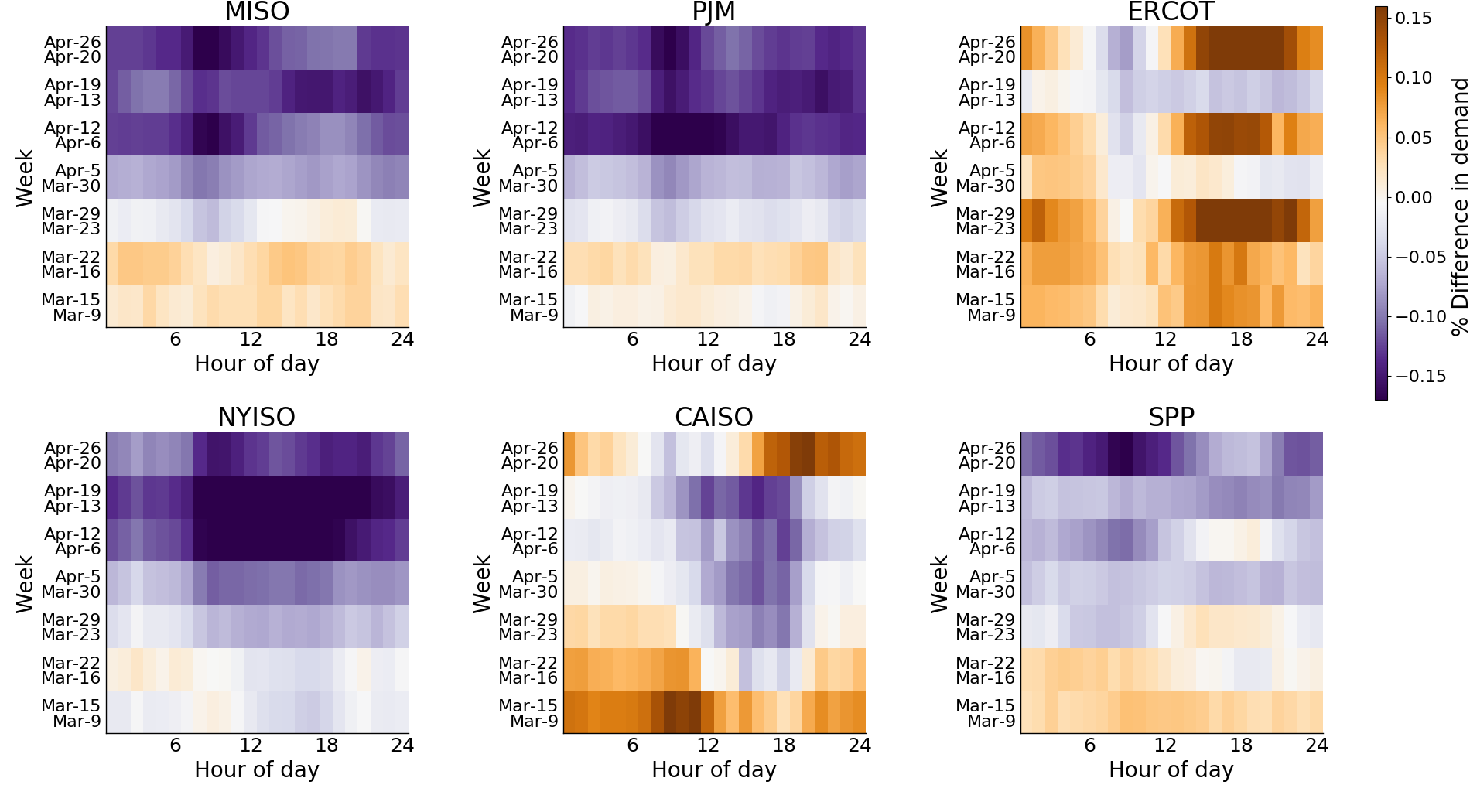 Figure 1: Percentage difference in demand by hour of day in March and April 2020 compared to 2019. A linear temperature adjustment has been applied to correct for demand reductions due to increases in temperature.
As was the case for many European countries, demand for electricity has decreased across most of the United States during April 2020 (Figure 1). Electricity demand recorded by the transmission operator for New York (NYISO) shows the largest decreases between the hours of 8am and 7pm, when many people would usually be either commuting or at their workplace. This data suggests that the decrease in industrial and commercial electricity demand from the closure of non-essential businesses, likely outweighs the increase in residential energy use we would expect now that many people are working from home.
For MISO and PJM, who oversee electricity systems in central and eastern states, we see reduced demand across April, with MISO showing the largest decline during the morning peak hours. The demand reported by the California Independent System Operator (CAISO) also shows reductions between the hours of 10am and 7pm. However, it is likely that a large part of this effect can be attributed to increases in behind-the-meter solar generation and less to do with the statewide lockdown. In Texas and the southwest, the figures reported by ERCOT and SPP break the trend and show increased demand over several weeks in April. Part of this increase is likely due to higher April temperatures in the south causing a rise in the use of residential air conditioning.
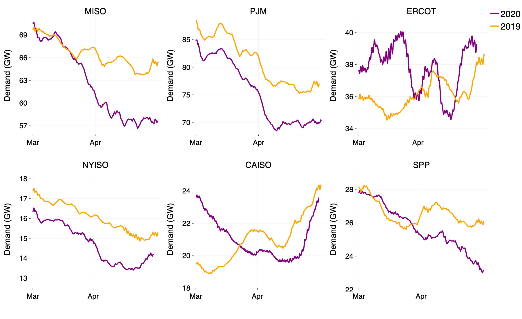 Figure 2: 7 day rolling average of electricity demand in March and April 2020 (purple), 2019 (orange).
Taking a step back to look at the long term trend in electricity demand (see Figure 2), we observe a clear turning point for some of the ISOs, coinciding with the order of statewide lockdowns. For MISO, and SPP, we see a similar demand for electricity during the majority of March, after which the demand this year begins plummeting in comparison to 2019 levels. In California, CAISO were initially reporting greater demand than in 2019, however, as restrictions were introduced during the latter half of March, a declining trend emerges which puts the 2020 demand well below what we saw last year. For the eastern ISOs, namely NYISO and PJM, the effect of lockdown on demand is less apparent, and in Texas, the demand reported by ERCOT in 2020 looks to be above the levels seen in 2019. Again, we can attribute much of this observed demand increase to a greater need for residential air conditioning, as the eastern and southern states have been experiencing a hot start to spring.
Whilst demand for electricity has decreased in the US, the effect of statewide lockdowns is not as striking as seen in Europe. This may be due to different states, which are overseen by the same ISO, introducing restrictions that vary in both severity and time of implementation, compared to the national lockdowns implemented in Europe. Nevertheless, daily patterns of energy consumption are far from the norm, and we next go on to explore how these changes are affecting electricity system planning.
How are the ISOs responding to the unusual changes to demand for electricity?
With the uncertainties in demand for electricity caused by statewide lockdowns, combined with the usual uncertainties inherent to the weather, demand forecasting for electricity has become more difficult for many of the ISOs. We find that this difficulty has led to considerably larger demand forecast errors (see Figure 3) than we have seen in previous years.
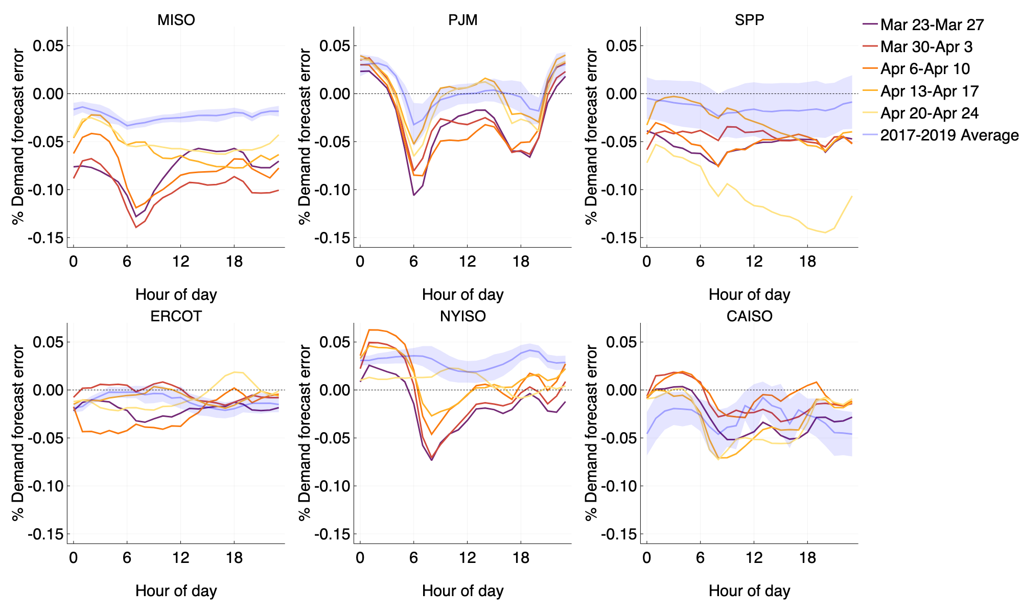 Figure 3: Hourly average weekday percent demand forecast error (\(\frac{\text{demand} - \text{forecast}}{\text{demand}}\)) over the final weeks in March and April. The 2017–2019 average over the same period is shown in blue.
The errors for MISO, PJM and NYISO clearly spike negative at 6am. This spike is due to over-forecasting the ramp up towards the morning peak demand, occurring around 9am/10am. With the shelter-in-place orders issued, these ISOs are struggling to adjust to the new morning patterns of a population now working at home. SPP looks to be less affected until the week beginning April 20th, when we see chronic over-forecasting throughout all hours of the day. This pattern is apparent in Figure 1, where the demand for electricity in SPP was relatively unaffected until the final two weeks of April.
How are these uncertainties affecting the efficiency of electricity systems?
As we discussed in the first post of this series, incorrect demand forecasts can reduce both the economic and environmental efficiency of electricity grids by causing divergence between the day ahead and real-time energy markets, and increasing the volume of energy curtailed to mitigate line congestion. Whilst we do not observe unusually large deviations between day ahead and real-time energy prices, we are seeing record breaking curtailment of combined wind and solar energy in California. Curtailment by CAISO has been growing year on year due to rising solar capacity, and previous reports indicated that this year would be no different.
Figure 4 (right) shows that curtailments in CAISO have reached ~300GWh in April 2020, soaring above the previous record of ~223GWh set in May 2019. To put this volume of curtailed energy into perspective, the average annual household consumption in the US is ~11,000kWh, which means the volume of curtailed renewable power in April is equivalent to the annual electricity usage of almost 30,000 homes. Looking at Figure 4 (left) we see that the volume of solar power produced in the first four months of 2020 is only marginally higher than the production levels seen in 2019. It is more likely that the combination of increased intermittent power production with decreased demand due to statewide lockdown, has forced CAISO to curtail more renewable power than ever before.
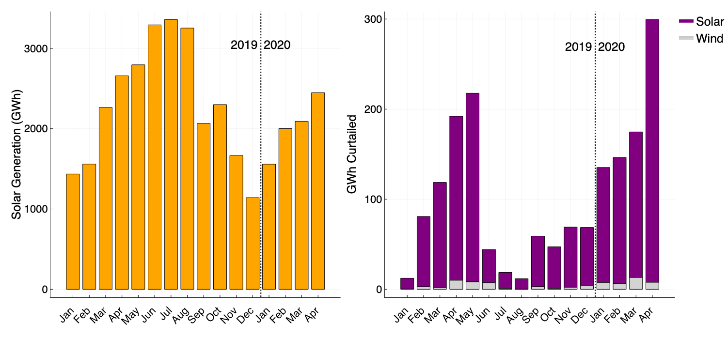 Figure 4: Left: monthly solar generation in CAISO, right: Solar and wind curtailments in CAISO throughout 2019 and 2020.
Growing curtailment of power has long been a concern for those in the control room at CAISO. This increase in wasted power highlights a lack of flexibility in the system in dealing with oversupply, and the effect of the current pandemic on reducing energy demand has amplified this further. To mitigate against additional growth in curtailment of renewable energy, and ensure less energy is wasted, utilities in California have set ambitious targets to increase grid storage capacity.
How is the generation mix changing to accommodate reduced demand?
As we saw in Europe, coal and gas based generation of electricity has declined due to national lockdowns. We find a similar pattern for PJM and MISO (see figure 5), where the hourly average production from coal has decreased ~7GW for both markets. Whilst some of this decrease is due to planned coal plant retirements making the way for cheaper generation technologies, the demand reductions we observe across the US are most likely to impact coal production before any other resource. This is because electricity markets are based on a type of auction, with the lowest cost generators receiving priority to serve demand. Coal powered generation is more expensive compared to natural gas and renewable production, which means coal power plants will be edged out of the auction when there is less demand for electricity.
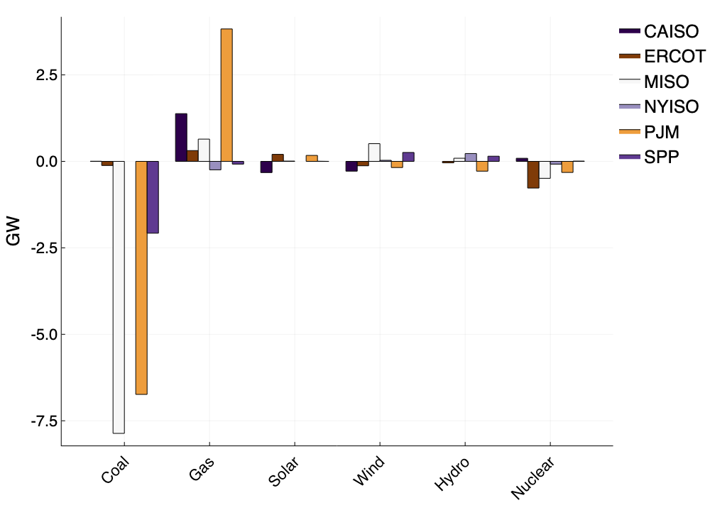 Figure 5: Average hourly change in production by fuel type between April 2020 and April 2019.
Looking at real time market wide energy prices, for most ISOs we can see that leading up to the outbreak of Covid-19, electricity prices were already down compared to 2019 levels (Figure 6). Coming into April, most ISOs had lower prices than at any time this year, and whilst prices continue to be low for some of the ISOs, an upwards trend emerges throughout the lockdown period.
The marketwide energy price is dependent on the least-cost generators available, and there are several factors, such as changing weather conditions and fluctuations in fuel supply, which can affect the generators available to serve demand. As an example, natural gas is one of the cheapest fuels for electricity generation. However, fluctuations in crude oil prices can have large impacts on the cost of natural gas generation, because a form of gas fuel, known as associated gas, is a by-product of crude oil. With the recent crash in oil prices where we saw negative oil futures for the first time in history, the production of associated gas has likely decreased throughout April. In the US, where close to 40% of generation is based on natural gas sources, a reduced supply of natural gas may be causing rises in electricity prices.
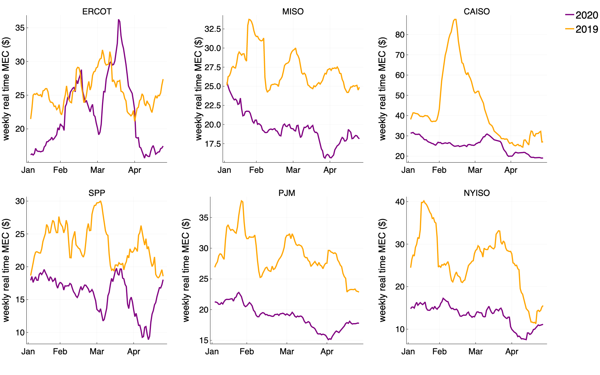 Figure 6: 7 day rolling average of the real time market-wide marginal energy cost for 2020 (purple) and 2019 (orange).
Conclusions
In this final post in our series, we have seen how electricity systems in the United States have responded to the changing patterns of electricity use induced by statewide lockdowns. We find demand forecasting has become more difficult for many of the ISOs, with CAISO forced to curtail record amounts of renewable power to manage oversupply and mitigate line overloading. Further, as was the case for Europe, we see coal generation taking the brunt of the decline in energy production, as lower cost generators are able to serve the depleted load. Finally, we explored how wholesale electricity prices have been affected by these changes. Whilst prices during lockdown have been the lowest seen this year, confounding factors such as the recent crash in oil prices may have led to rising wholesale electricity prices throughout April.
17 Apr 2020
Author: Ian Goddard
In Part 1 of this series on how national lockdowns have affected electricity markets and system operations, we discussed how declining demand has changed the daily patterns of electricity usage in Europe, and the challenges this brings to electricity system operators.
With Covid-19 continuing to cause widespread shutdown of businesses and public institutions around the world, we are seeing a marked decrease in the demand for electricity ,.
In this post we will explore how the different types of power generation in several European countries are being affected by declining energy demand, and how this may be affecting pollutant emissions from European electricity systems.
Furthermore, we will see how oversupply of energy, due to reductions in demand, is affecting wholesale energy market prices.
How have national lockdowns affected electricity production?
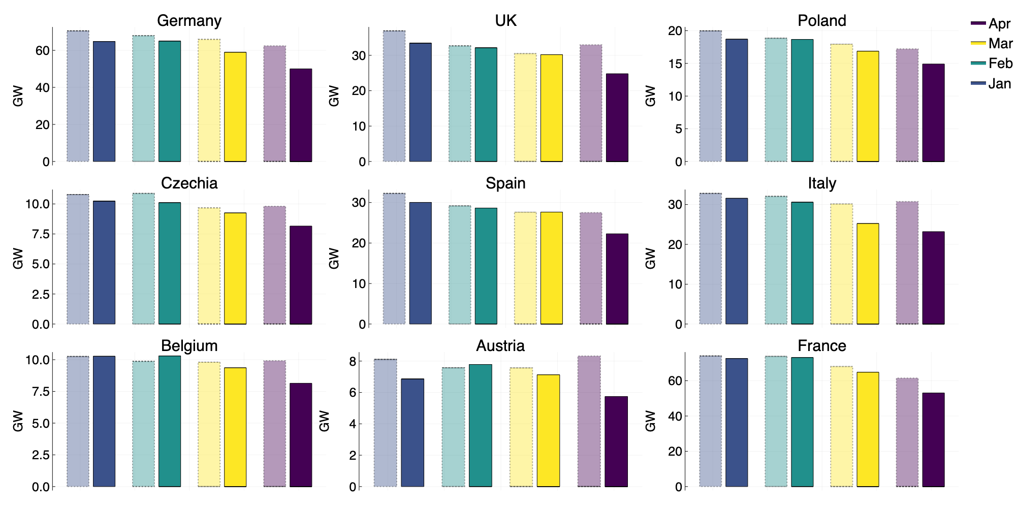 Figure 1: Average hourly electricity generation from all sources in the first 4 months of 2020 (solid), and 2019 (faint).
Looking at the average hourly electricity generation per month (Figure 1), we observe a significant decline in energy production compared to 2019 for both March and April.
The generation of electricity comes from various sources, such as nuclear or coal power plants, defining what is called the generation fuel mix.
Given the striking decline in overall generation, the question arises of how this affects the generation fuel mix.
First, however, there is another important factor that influences electricity demand, and therefore generation.
Demand for electricity is weather-dependent and, after a relatively mild winter and an early spring, it is reasonable to consider that a portion of the reduction in demand may be due to increased temperatures.
In our analysis we are concerned with the temperature differences between the early spring of 2020 and the same period in 2019.
Differences between European temperature anomalies for March 2019 and March 2020, are approximately 1˚C, and, as mentioned in part 1, a high estimate of the effect of temperature on demand is of 1.5-2.0% decrease per 1˚C temperature increase.
After accounting for temperature effects, there are still differences in the generation fuel mix that suggest effects from the demand reductions caused by nationwide lockdowns.
In order to understand this, we must first review the dynamics of the generation fuel mix during normal circumstances.
Typically, an increase in generation from renewable sources, such as wind and solar, leads to decreases in production from fossil fuels, most often from natural gas or coal.
Looking at the data for Germany in February (Figure 2), we see roughly a 5GW decrease from both hard and brown coal generation.
However, this is accompanied by a staggering ~10GW increase in wind generation.
We see a similar situation for the UK, where ~4GW of wind generation has displaced gas production in both January and February of 2020.
An indication of an overall decrease in demand is a reduction in generation from one power source that is not compensated by an increase in generation from other sources.
This is precisely what we observe for many countries in April 2020.
Hard and brown coal generation in Germany once again show a ~5GW decrease, yet there is no increase in production from any other source.
The UK has seen a ~5GW drop in gas production, with no renewable generation to replace these losses.
Italy, Belgium and France also show large reductions in gas generation, whilst the Czech Republic, and Poland see reductions in brown and hard coal respectively.
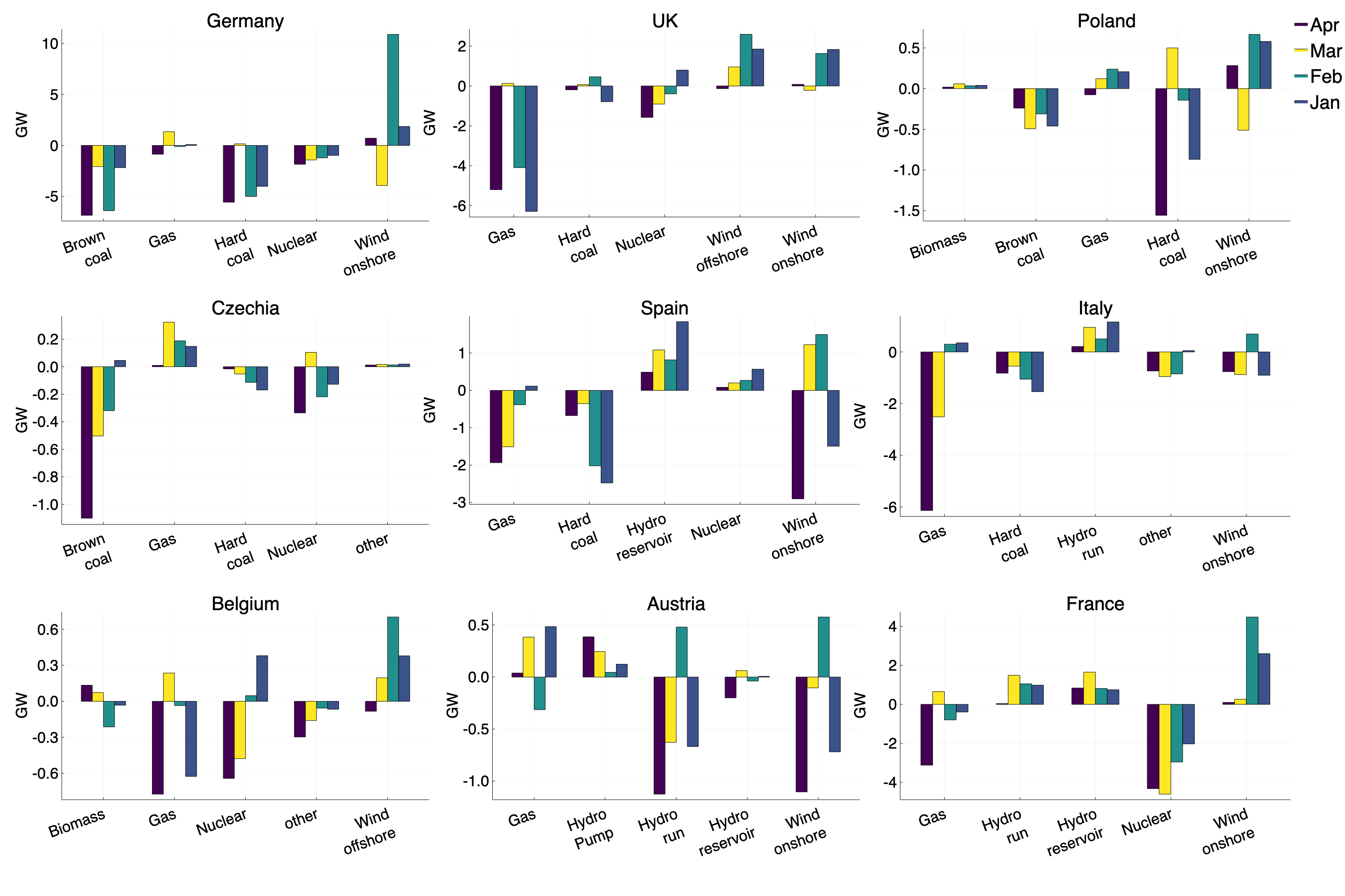 Figure 2: Difference in average hourly generation by fuel type between 2020 and 2019 by month.
We only discuss the top 5 contributors to the energy mix, as these have the most impact.
Figure 2: Difference in average hourly generation by fuel type between 2020 and 2019 by month.
We only discuss the top 5 contributors to the energy mix, as these have the most impact.
How might this be affecting carbon emissions of European electricity systems?
Given the reductions in gas and coal production as a result of decreased demand caused by national lockdowns, we can estimate the effect of lockdowns on emissions produced by electricity generation.
In order to make such estimates we use what is known emissions factors for each fuel type.
The emissions factor for a fuel type tells us the mass of carbon dioxide emitted per kilowatt-hour (kWh) of energy produced using that fuel.
Detailed emission factors can be found here but for our rough estimates we use values of \(0.2\ kg CO_2 / kWh\) and \(0.3\ kg CO_2 / kWh\) for natural gas and brown/hard coal, respectively.
Taking Italy as an illustrative example, where lockdown has been in place for the majority of March and April, we see an average decrease of ~4GW in hourly gas generation (across both months).
Thus, the hourly reduction in emissions is given by the emissions factor for gas (\(E_g\)) multiplied by the reduction in generation (\(G_r\)) .
\begin{align}
E_g \times G_r & = 0.2\ kg CO_2 / kWh \times \text{4,000,000}\ kW \nonumber \\
& = \text{800,000}\ kg CO_2 /h \nonumber
\end{align}
Our estimate comes to an average of 800 tonnes less of \(CO_2\) emissions for every hour during lockdown.
If we assume these restrictions will last for 8 weeks (1344 hours), the total reduction over the whole lockdown period would be ~1.1M tonnes.
To put this into perspective, the annual average emissions per capita in Europe is ~6 tonnes, meaning the reductions observed over the 8 weeks, are equivalent to the yearly emissions of ~180,000 people.
Applying the same method across all countries, we see that national lockdowns across Europe have reduced \(CO_2\) emissions from electricity generation equivalent to the annual emissions of nearly 1 million people (Table 1), or roughly 6M tonnes.
Our analysis shows how reductions in electricity generation will play a role in making 2020 a record year for reducing carbon emissions.
Table 1: Reductions in emissions for each country due to the decline in electricity production by fuel type. Note that we see no significant reduction in the fossil based generation in Austria.
| Country |
Reduction in gas (GW) |
Reduction in coal (GW) |
CO2 emissions saved (Mt) |
Equivalent number of people |
| Italy |
~4 |
- |
1.1 |
215000 |
| Spain |
~1.5 |
- |
0.4 |
67000 |
| France |
~3 |
- |
0.81 |
134000 |
| Germany |
- |
~4 |
1.61 |
268000 |
| Poland |
- |
~1 |
0.4 |
67000 |
| Czechia |
~0.7 |
- |
0.19 |
31000 |
| Austria |
- |
- |
- |
- |
| Belgium |
~0.6 |
- |
0.16 |
27000 |
| UK |
~2.5 |
- |
0.67 |
112000 |
How has this changed the overall energy mix and how might this be affecting electricity markets?
Overall, the declining power demand is having a disproportionate effect on power generation from fossil fuels.
We see a stark effect in Italy, where non-fossil sources are now serving over half of the demand, compared to less than 40% seen in previous months.
In the UK and Germany, the percentage of generation from non-fossil sources is on par with what we saw during in February, where both countries saw huge surges in wind power generation.
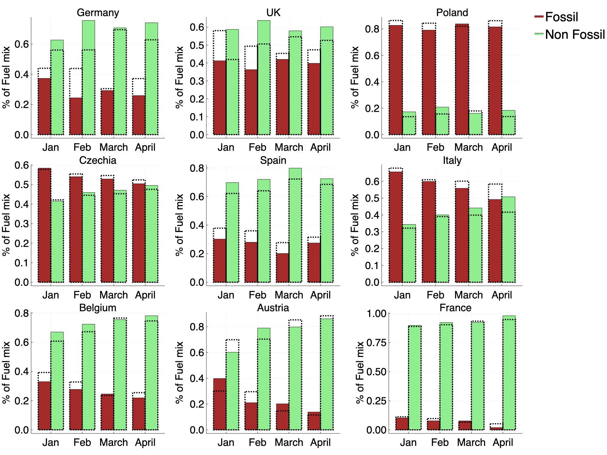 Figure 3: Hourly average percentage of the fuel mix for both fossil (brown) and non fossil sources (green). The 2019 values are indicated by the dotted lines.
Combining a high percentage of renewable energy output, with a drastic reduction in electricity demand creates an unusual situation for electricity system operators.
The variability in renewable generation coupled with unprecedented reductions in the demand for electricity, creates a situation where generation plants may have to pay to provide electricity, as opposed to being paid to do so.
In many European electricity markets, the price for unplanned electricity supply or demand is known as the imbalance price.
In almost all cases, the imbalance price is positive, where generators are paid to provide power to ensure supply meets the demand.
However, when there is an overwhelming surplus of power, the imbalance price can fall below zero.
In such cases, electricity system operators set negative imbalance prices to motivate generators to halt production, by forcing them to pay to provide electricity.
During March and April, we see spikes in the frequency of negative imbalance prices in several European countries (Figure 4), indicating that there is a large surplus of available power and less incentive for suppliers to generate electricity.
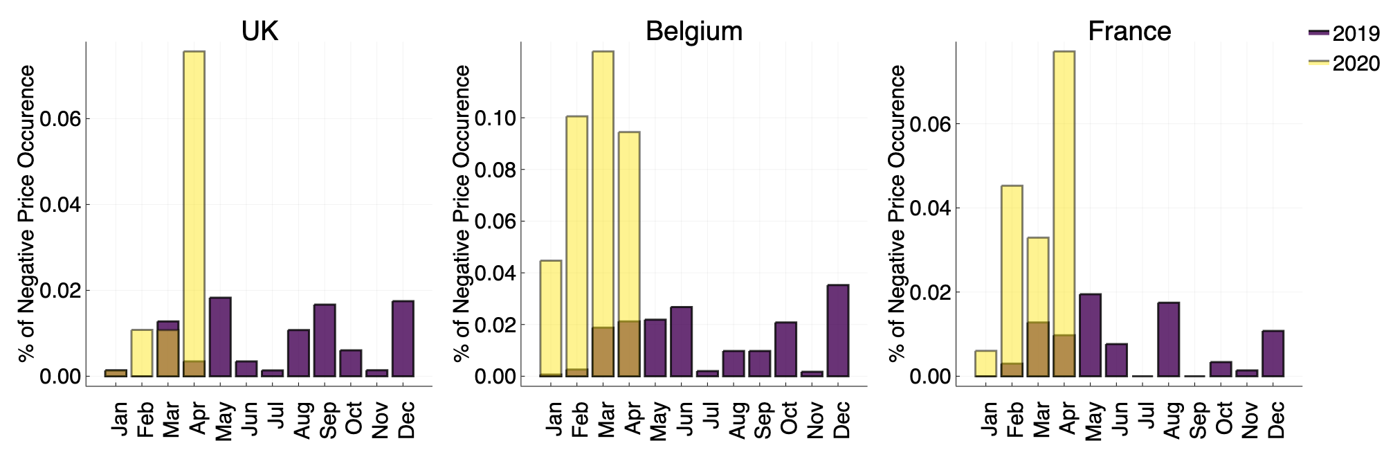 Figure 4: Percentage of negative imbalance prices per month for 2019 (blue) and 2020 (yellow).
Conclusions
In the second part of this series, we have explored how restrictions due to Covid-19 have affected the generation mix of several European countries.
We find a disproportionate reduction to the output from both coal and gas power plants and estimate a decline in carbon emissions equivalent to that of the annual emissions of nearly 1 million people.
Furthermore, the impact of reduced fossil generation has led some countries to see a cleaner energy mix than normal, which, combined with record low demand, has led to electricity system operators acting to disincentivize the production of electricity.
In part 3, we will look at the United States, to see how electricity systems there are changing in the country currently hit hardest by Covid-19.
31 Mar 2020
Author: Ian Goddard
In the midst of the ongoing global coronavirus crisis, management and accurate planning of electricity grids is all the more important, in order to reduce the risk of blackouts and ensure power can be supplied to crucial industries.
With an ever-growing estimate of 1.7 billion people under some form of lockdown as of March 24th, the usual daily patterns of electricity usage across the world have been changing dramatically.
Already, we have seen reports showing that electricity demand across Europe has drastically decreased since it became the epicentre of the pandemic.
One might think that excess supply of electricity can’t be a bad thing, however, electrical grid management is a careful balancing process where energy supply must equal demand at all times.
Oversupply of electricity can cause transmission line overloading, and if managed incorrectly this may have drastic consequences.
We had a look at some data from European and American electricity grid operators, and in a series of posts we will try to answer the following questions:
1) Have there been any interesting changes in daily patterns of energy usage, other than notable decline?
2) Could forecasting of daily electricity demand be more difficult now that so many people are working from home?
3) With reduced generation required to meet demand, how are the energy source mix and pollutant emissions affected?
To what extent are lockdown restrictions affecting the amount of electricity we use?
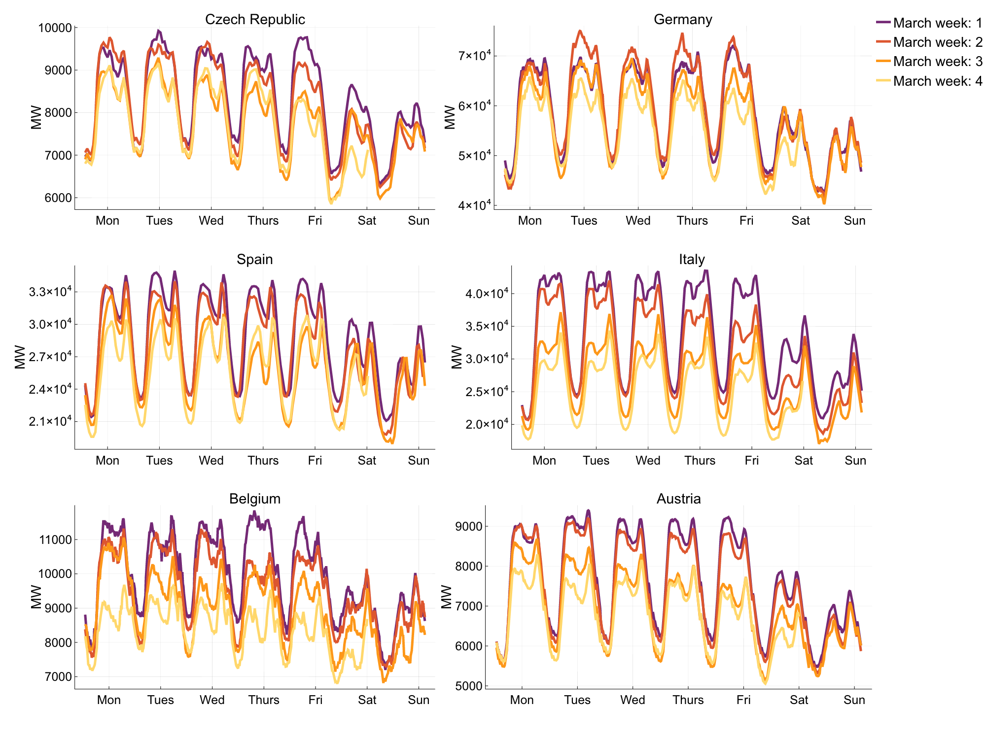 Figure 1: Week on Week electricity demand in March 2020 .
As we can see from the plots in Figure 1, demand for electricity across many European countries has experienced a drastic decrease, week after week, throughout the whole of March.
People who normally commute to and from work are instead staying home, so we might expect the weekday demand would look similar to the weekend demand, as office buildings, schools, and universities are closed. Looking at Figure 1, it is clear that as the lockdown measures continue, we begin to see these large reductions in peak weekday demand. This decline is particularly apparent in Italy, where strict lockdown measures have been in place for several weeks. By the 4th week of March, the peak weekday demand in Italy has fallen below the peak weekend demand seen in the first week of March. It’s likely the usual peak weekend demand is greater than current weekday demand due to the closure of many businesses, such as restaurants, bars, and galleries, which often see the most activity during weekends.
To clarify, our plots have not been adjusted for temperature changes in March. It’s important to note that whilst electricity demand is weather dependent, it’s clear that the changes we see in demand are not solely due to gradual temperature increase throughout March.
A high estimate of the effect of temperature would be 1.5-2% demand change per 1°C.
In many countries, we observe ~20% demand decrease which would correspond to a 10°C change in temperature. The large declines in demand that we observe are more consistent with school/business closures during holiday periods, as we would expect given the current restrictions in place in many European countries.
How might we expect national lockdowns to affect daily demand profiles?
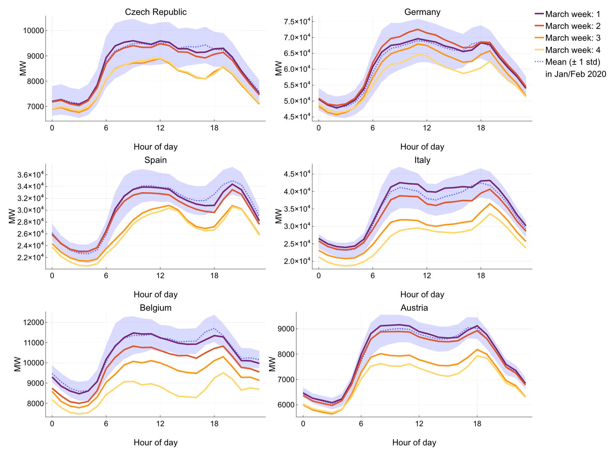 Figure 2: Hourly electricity demand profile, averaged over weekdays for each week in March (coloured), and all weeks leading up to March (black/blue).
Looking at the hourly electricity demand, averaged over weekdays for each week in March, and comparing to the hourly demand averaged for all weeks in 2020 leading up to March, we see several notable differences (see Figure 2).
Other than the prominent decline in peak demand as the weeks progress, the morning peak in Spain and the Czech Republic has been shifted later by several hours.
It’s possible that people are starting their workday later now that they no longer have to commute.
Interestingly, in Italy there is an inversion of the demand curve, where the evening peak, driven by residential lighting, heating, and cooking, is pushed higher than the morning peak.
With these changes in mind, how might grid operators be coping with these unusual shifts in daily usage patterns?
In Figure 3, we can see the hourly percentage demand forecast error averaged over weekdays for each week in March.
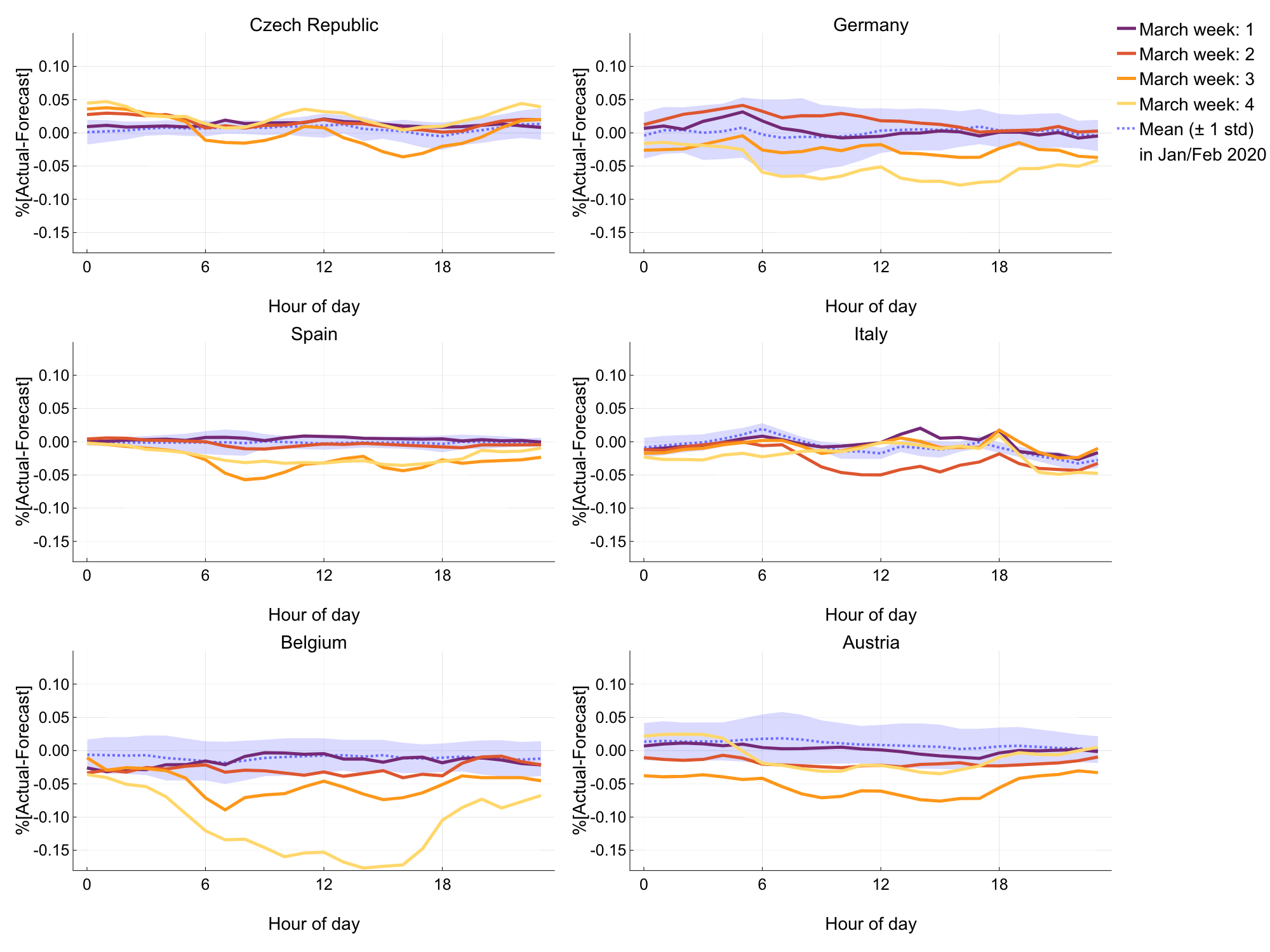 Figure 3: Hourly percentage demand forecast error, averaged over weekdays in each week of March (coloured), and all subsequent weeks leading up to March (black/blue).
Comparing to the distribution of hourly percentage forecast errors for all weeks in 2020 up until March, we see some striking differences.
It’s clear that the latter half of March has proven difficult to forecast for transmission system operators (TSOs), due to the unusual changes in daily energy use.
It’s likely that this has increased congestion in electricity grids across Europe, as TSOs are planning for higher loads than are seen in real time.
Planning to provide more power than is required leads to over-commitment of energy resources which increases the economic and environmental cost of electricity markets, as congestion prices increase and renewable energy is curtailed to prevent transmission line overloading.
It will be interesting to see how long it takes for TSOs to adjust to the new norms in daily energy use.
Conclusions
In part 1 of this series, we’ve explored electricity demand data for several European countries and how the restrictions imposed to limit the impact of coronavirus are affecting both usage of electricity and TSO planning.
Not only is there a clear decline in electricity demand, we also observe notable changes in daily demand profiles, indicating a marked shift in the peak hours for electricity usage. In addition to this, we’ve seen that such drastic and uncertain changes in when and how much power will be consumed have caused forecasting problems for transmission system operators, which may be reducing economic and environmental efficiency in European electricity systems.
In part 2, we’ll explore how changes in electricity demand have affected the energy mix in Europe, and whether or not this has affected the overall emissions of European electricity systems.
24 Jan 2020
Author: Invenia team

Introduction
In early December 2019, part of the Invenia team headed to Vancouver, Canada, for the annual Neural Information Processing Systems (NeurIPS, previously NIPS) conference. It was the biggest NeurIPS conference yet, with an estimated 13,000 attendees, 6,743 paper submissions, and almost 80 official meetups.
We sent developers, researchers, and people operation representatives from both Cambridge and Winnipeg to attend talks, meet people, and run our booth at the expo. Below are some of our highlights from the week.
Yoshua Bengio and Blaise Aguera y Arcas Keynotes
The keynote talks by Blaise Aguera y Arcas and Yoshua Bengio offered interesting perspectives and discussed a new, or arguably old, direction for the learning community. Bengio outlined how current deep learning is excelling with “system 1 learning”, tasks that we as humans do quickly and unconsciously. At the same time, Aguera y Arcas discussed AI’s superhuman performance in such tasks. Punctuating the message of both talks, Aguera y Arcas described just how little territory this covers if we are interested in building a more human-like intelligence.
Current learning methods are lacking in what Bengio refers to as “system 2 learning” - slow, conscious, and logical problem-solving. He underlined some of the missing pieces of current deep learning, such as better out-of-distribution generalisation, high-level semantic representation, and an understanding of causality. The notion that state-of-the-art methods may be inadequate seemed even clearer when Aguera y Arcas questioned whether natural intelligence ever performs optimisation. He highlighted that “evolution decides on what is good and bad” rather than having some predefined loss to optimise.
It’s interesting to see that, even after the many recent advances in deep learning, we are still at a loss when it comes to replicating a natural form of intelligence – which was the initial motivation for neural networks. Both speakers addressed meta-learning, a prominent research area at NeurIPS this year, as a step in the right direction. However, the concluding message from Aguera y Arcas was that, to build natural intelligence, we may need to explore brains with evolved architectures, cellular automata, and social or cooperative learning among agents.
On a completely unrelated note, Blaise Aguera also mentioned a great comic on the nascent field of federated learning. For anyone not familiar with the term, it’s a cute introduction to the topic.
Tackling Climate Change with Machine Learning
Among the workshops, this year’s “Tackling Climate Change with Machine Learning” was particularly interesting for us.
Jeff Dean from Google AI gave an interesting talk about using Bayesian inference for physical systems. One such application discussed was using TensorFlow Probability to help stabilize the plasma flows in a type of fusion reactor. Another topic was on using TPUs for simulating partial differential equations, such as hydraulic model simulation for flood forecast, and combining the results with neural nets for weather prediction. He also mentioned that Google data centers are “net zero-carbon” since 2017. However, this does not mean they consume no fossil fuels – they offset that consumption by producing renewable energy which is then made available to the grid – so there is still room for improvement.
In addition to this, Qinghu Tang discussed the use of semi-supervised learning to create a fine-grained mapping of the low voltage distribution grid using street view images. Their ambitious plan is to create “a comprehensive global database containing information on conventional and renewable energy systems ranging from supply, transmission, to demand-side.” This announcement is particularly exciting to those using cleaner energy sources to combat climate change, as this database would be largely useful for planning.
Earlier in 2019, at the ICML 2019 Workshop, we presented a poster in which we proposed an algorithm for reducing the computational time of solving Optimal Power Flow (OPF) problems. As a follow-up we presented another poster, in which we apply meta-optimisation in combination with a classifier that predicts the active constraints of the OPF problem. Our approach reduces the computational time significantly while still guaranteeing feasibility. A promising future direction is to combine it with the work of Frederik Diehl using graph neural networks (GNN) for predicting the solution of AC-OPF problems.
Responsible use of computing resources
On the last day of the conference, the Deep Reinforcement Learning (RL) panel was asked about the responsible use of computing resources. The answers highlighted the many different stances on what can be a contentious matter.
Some showed a sense of owing the community something, realising that they are in a privileged position, and choosing wisely which computationally expensive experiments to run.
It was also mentioned that there is a need to provide all parts of the community with access to extensive computing resources, instead of just a few privileged research teams in a handful of industry labs.
However, the challenge lies in how to achieve that.
A different point of view is that we should not be convinced that all research requires large amounts of computing resources. Novel research can still be done with tabular environment reinforcement learning experiments, for instance. It is important to avoid bias towards compute-heavy research.
There have been some attempts at limiting the available resources, in hopes of sparking new research insights, but we still have to see the results of this initiative. Ultimately, there are cases in which the adoption of compute-heavy approaches might simply be unavoidable, such as for reinforcement learning in large continuous control tasks.
Advances in Approximate Bayesian Inference (AABI) Workshop
One of the hidden gems of NeurIPS is the co-located workshop Advances in Approximate Bayesian Inference (AABI), which provides a venue for both established academics as well as more junior researchers to meet up and discuss all things Bayesian. This year the event was the largest to-date - with 120 accepted papers compared to just 40 last year - and consisted of 11 talks and two poster sessions, followed by a panel discussion.
Sergey Levine, from UC Berkeley discussed the mathematical connections between control and Bayesian inference (aka control-as-inference framework). More specifically, Levine presented an equivalence between maximum-entropy reinforcement learning (MaxEnt RL) and inference in a particular class of probabilistic graphical models. This highlighted the usefulness of finding a principled approach to the design of reward functions and addressing the issue of robustness in RL.
In the poster session, we presented GP-ALPS, our work on Bayesian model selection for linear multi-output Gaussian Process (GP) models, which find a parsimonious, yet descriptive model. This is done in an automated way by switching off latent processes that do not meaningfully contribute to explaining the data, using latent Bernoulli variables and approximate inference.
The day finished with a panel discussion that featured, among others, Radford Neal and James Hensman.
The participants exchanged opinions on where Bayesian machine learning can add value in the age of big data and deep learning, for example, on tasks that require reasoning about uncertainty.
They also discussed the trade-offs between modern Monte Carlo techniques and variational inference, as well as pointed out the current lack of standard benchmarks for uncertainty quantification.
Dealing with real-world data
It was nice to see some papers that specifically looked at modelling with asynchronous and incomplete data, data available at different granularities, and dataset shift - all scenarios that arise in real-world practice. These interesting studies make a refreshing change from the more numerous papers on efficient inference in Bayesian learning and include some fresh, outside-the-box ideas.
GPs were widely applied in order to deal with real-world data issues. One eye-catching poster was Modelling dynamic functional connectivity with latent factor GPs. This paper made clever use of transformations of the approximated covariance matrix to Euclidean space to efficiently adapt covariance estimates. A paper that discussed the problem of missing data in time-series was Deep Amortized Variational Inference for Multivariate Time Series Imputation with Latent Gaussian Process Models. There were also papers that looked at aggregated data issues such as Multi-task learning for aggregated data using Gaussian processes, Spatially aggregated Gaussian processes with multivariate areal outputs, and Multi-resolution, multi-task Gaussian processes. The latter contained some fancy footwork to incorporate multi-resolution data in a principled way within both shallow and deep GP frameworks.
Naturally, there were also several unsupervised learning works on the subject. A highlight was Sparse Variational Inference: Bayesian coresets from scratch, presenting the integration of data compression via Bayesian coresets in SVI with a neat framework for the exponential family. Additionally, the paper discussing Multiway clustering via tensor block modules, presented an algorithm for clustering in high-dimensional feature spaces, with convergence and consistency properties set out clearly in the paper. Finally, we must mention Missing not at random in matrix completion: the effectiveness of estimating missingness probabilities under a low nuclear norm assumption, a paper that proposes a principled approach to filling in missing data by exploiting an assumption that the ‘missingness’ process has a low nuclear norm structure.
Research engineering
Research Engineering is often overlooked in academic circles, even though this is a key role in most companies doing any amount of machine learning research. NeurIPS was a good venue for discussion with research engineers from several companies, which provided some interesting insights into how workflow varies across industry. We all had lots of things in common, such as figuring out how to match research engineers to research projects and trying to build support tools for everyday research tasks.
In many companies, the main output is often research (papers, not products), and having the same people who do novel research resulting in papers also work on putting machine learning into production seemed surprisingly rare. This choice can lead to the significant problem of having two different languages – for example, PyTorch for researchers and TensorFlow for production – which causes extra strain on research engineers who become responsible for translating code and dealing with language particularities. We are fortunate to avoid this kind of issue, both by enforcing high standards on code written by researchers, but more importantly having research code never too far from being able to run in production.
Research Retrospectives
A new addition to the workshops this year was Retrospectives in Machine Learning . The core idea of a retrospective is to reflect on previous work and to discuss shortcomings in the initial intuition, analysis, or results. The goal of the workshop was to “improve the science, openness, and accessibility of the machine learning field, by widening what is publishable and helping to identify opportunities for improvement.” In a way, we can say that it discusses which things readers of important papers should know now, that were not in the original publication.
There were many great talks, with one of the most honest and direct discussions being David Duvenaud’s “Bullshit that I and others have said about Neural ODEs”. The talk discussed many insights on the science side, as well as around what happened after the Neural ODEs paper was published at NeurIPS 2018. An overarching theme of the talk is the sociology of the very human institutions of research. As an example, the talk suggests thinking about how science journalists have distinct incentives, how these interact with researcher/academic incentives, and how this can – even inadvertently – result in hype.
The program transformations workshop was primarily focused on automatic differentiation (AD), which has been a key element in the development of modern machine learning techniques.
The workshop was a good size, with a substantial portion of all people who are currently doing interesting things in AD, such as Jax, Swift4TF and ChainRules.jl in attendance.
Also present were some of the fathers of AD, such as Laurent Hascoët and Andreas Griewank.
Their general attitude towards recent work seemed to be that there have not been significant theoretical advances since the ‘80s.
Still, there has been considerable progress toward making AD more useful and accessible.
One of the major topics was AD theory: the investigation of the mathematical basis of current methods. As a highlight, the Differentiable Curry presentation introduced a diagrammatic notation which made the type-theory in the original paper much clearer and more intuitive.
Various new tools were also presented, such as Jax, which made its first public appearance at a major conference.
There have been many Jax-related discussions in the Julia community, and it seems to be the best of all Python JITs for differentiable programming. Also of note was Torchscript, a tool that allows running Pytorch outside of Python.
There were also more traditional AD talks, such as high-performance computing (HPC) AD in Fortran and using MPI. A nice exception was Jesse Bettencourt’s work on Taylor-Mode Automatic Differentiation for Higher-Order Derivatives, which is an implementation of Griewank and Walther (2008) chapter 13 in Jax.
Conclusion
As usual, NeurIPS represents a great venue to stay connected with the newest advances and trends in the most diverse subfields of ML. Both academia and industry are largely represented, and that creates an unique forum. We look forward to joining the rest of the community again in the upcoming NeurIPS 2020 and invite everyone to stop by our booth and meet our team.
06 Nov 2019
Author: Frames Catherine White
Introduction
This blog post is based on a talk originally given at a Cambridge PyData Meetup, and also at a London Julia Users Meetup.
This is the second of a two-part series of posts on the Emergent Features of JuliaLang.
That is to say, features that were not designed, but came into existence from a combination of other features.
While Part I was more or less a grab-bag of interesting tricks,
Part II (this post), is focused solely on traits, which are, in practice, much more useful than anything discussed in Part I.
This post is fully indepedent from Part I.
Traits
Inheritance can be a gun with only one bullet, at least in the case of single inheritance like Julia uses.
Single-inheritance means that, once something has a super-type, there can’t be another.
Traits are one way to get something similar to multiple inheritance under such conditions.
They allow for a form of polymorphism,
that is orthogonal to the inheritence tree, and can be implemented using functions of types.
In an earlier blog post this is explained using a slightly different take.
Sometimes people claim that Julia doesn’t have traits, which is not correct.
Julia does not have syntactic sugar for traits, nor does it have the ubiqutious use of traits that some languages feature.
But it does have traits, and in fact they are even used in the standard library.
In particular for iterators, IteratorSize and IteratorEltype, and for several other interfaces.
These are commonly called Holy traits, not out of religious glorification, but after Tim Holy.
They were originally proposed to make StridedArrays extensible.
Ironically, even though they are fairly well established today, StridedArray still does not use them.
There are on-going efforts
to add more traits to arrays, which one day will no doubt lead to powerful and general BLAS-type functionality.
There are a few ways to implement traits, though all are broadly similar.
Here we will focus on the implementation based on concrete types.
Similar things can be done with Type{<:SomeAbstractType} (ugly, but flexible),
or even with values if they are of types that constant-fold (like Bool),
particularly if you are happy to wrap them in Val when dispatching on them (an example of this will be shown later).
There are a few advantages to using traits:
- Can be defined after the type is declared (unlike a supertype).
- Don’t have to be created up-front, so types can be added later (unlike a
Union).
- Otherwise-unrelated types (unlike a supertype) can be used.
A motivating example from Python: the AsList function
In Python TensorFlow, _AsList is a helper function:
def _AsList(x):
    return x if isinstance(x, (list, tuple)) else [x]
This converts scalars to single item lists, and is useful because it only needs code that deals with lists.
This is not really idiomatic python code, but TensorFlow uses it in the wild.
However, _AsList fails for numpy arrays:
>>> _AsList(np.asarray([1,2,3]))
[array([1, 2, 3])]
This can be fixed in the following way:
def _AsList(x):
    return x if isinstance(x, (list, tuple, np.ndarray)) else [x]
But where will it end? What if other packages want to extend this?
What about other functions that also depend on whether something is a list or not?
The answer here is traits, which give the ability to mark types as having particular properties.
In Julia, in particular, dispatch works on these traits.
Often they will compile out of existence (due to static dispatch, during specialization).
Note that at some point we have to document what properties a trait requires (e.g. what methods must be implemented).
There is no static type-checker enforcing this, so it may be helpful to write a test suite for anything that has a trait which checks that it works properly.
The Parts of Traits
Traits have a few key parts:
- Trait types: the different traits a type can have.
- Trait function: what traits a type has.
- Trait dispatch: using the traits.
To understand how traits work, it is important to understand the type of types in Julia.
Types are values, so they have a type themselves: DataType.
However, they also have the special pseudo-supertype Type, so a type T acts like T<:Type{T}.
typeof(String) === DataType
String isa Type{String} === true
String isa Type{<:AbstractString} === true
We can dispatch on Type{T} and have it resolved at compile time.
Trait Type
This is the type that is used to attribute a particular trait.
In the following example we will consider a trait that highlights the properties of a type for statistical modeling.
This is similar to the MLJ ScientificTypes.jl, or the StatsModel schema.
abstract type StatQualia end

struct Continuous <: StatQualia end
struct Ordinal <: StatQualia end
struct Categorical <: StatQualia end
struct Normable <: StatQualia end
Trait Function
The trait function takes a type as input, and returns an instance of the trait type.
We use the trait function to declare what traits a particular type has.
For example, we can say things like floats are continuous, booleans are categorical, etc.
statqualia(::Type{<:AbstractFloat}) = Continuous()
statqualia(::Type{<:Integer}) = Ordinal()

statqualia(::Type{<:Bool}) = Categorical()
statqualia(::Type{<:AbstractString}) = Categorical()

statqualia(::Type{<:Complex}) = Normable()
Using Traits
To use a trait we need to re-dispatch upon it.
This is where we take the type of an input, and invoke the trait function on it to get objects of the trait type, then dispatch on those.
In the following example we are going to define a bounds function, which will define some indication of the range of values a particular type has.
It will be defined on a collection of objects with a particular trait, and it will be defined differently depending on which statqualia they have.
using LinearAlgebra

# This is the trait re-dispatch; get the trait from the type
bounds(xs::AbstractVector{T}) where T = bounds(statqualia(T), xs)

# These functions dispatch on the trait
bounds(::Categorical, xs) = unique(xs)
bounds(::Normable, xs) = maximum(norm.(xs))
bounds(::Union{Ordinal, Continuous}, xs) = extrema(xs)
Using the above:
julia> bounds([false, false, true])
2-element Array{Bool,1}:
 false
 true

julia> bounds([false, false, false])
1-element Array{Bool,1}:
 false

julia> bounds([1,2,3,2])
(1, 3)

julia> bounds([1+1im, -2+4im, 0+-2im])
4.47213595499958
We can also extend traits after the fact: for example, if we want to add the
property that vectors have norms defined, we could define:
julia> statqualia(::Type{<:AbstractVector}) = Normable()
statqualia (generic function with 6 methods)

julia> bounds([[1,1], [-2,4], [0,-2]])
4.47213595499958
Back to AsList
First, we define the trait type and trait function:
struct List end
struct Nonlist end

islist(::Type{<:AbstractVector}) = List()
islist(::Type{<:Tuple}) = List()
islist(::Type{<:Number}) = Nonlist()
Then we define trait dispatch:
aslist(x::T) where T = aslist(islist(T), x)
aslist(::List, x) = x
aslist(::Nonlist, x) = [x]
This allows aslist to work as expected.
julia> aslist(1)
1-element Array{Int64,1}:
 1

julia> aslist([1,2,3])
3-element Array{Int64,1}:
 1
 2
 3

julia> aslist([1])
1-element Array{Int64,1}:
 1
As discussed above this is fully extensible.
Dynamic dispatch as fallback.
All the traits discussed so far have been fully-static, and they compile away.
We can also write runtime code, at a small runtime cost.
The following makes a runtime call to hasmethod to look up if the given type
has an iterate method defined.
(There are plans to make hasmethod compile time.
But for now it can only be done at runtime.)
Similar code to this can be used to dispatch on the values of objects.
islist(T) = hasmethod(iterate, Tuple{T}) ? List() : Nonlist()
We can see that this works on strings, as it does not wrap the following into an array.
julia> aslist("ABC")
"ABC"
Traits on functions
We can also attach traits to functions, because functions are instances of singleton types,
e.g. foo::typeof(foo).
We can use this idea for declarative input transforms.
As an example, we could have different functions expect the arrangement of observations to be different.
More specifically, different machine learning models might expect the inputs be:
- Iterator of Observations.
- Matrix with Observations in Rows.
- Matrix with Observations in Columns.
This isn’t a matter of personal perference or different field standards;
there are good performance-related reasons to choose one the above options depending on what operations are needed.
As a user of a model, however, we should not have to think about this.
The following examples use LIBSVM.jl, and DecisionTree.jl.
In practice we can just use the MLJ interface instead,
which takes care of this kind of thing.
In this demonstration of the simple use of a few ML libraries, first we need some basic functions to deal with our data.
In particular we want to define get_true_classes which as it would naturally be written would expect an iterator of observations.
using Statistics
is_large(x) = mean(x) > 0.5
get_true_classes(xs) = map(is_large, xs)

inputs = rand(100, 1_000);  # 100 features, 1000 observations
labels = get_true_classes(eachcol(inputs));
For simplicity, we will simply test on our training data,
which should be avoided in general (outside of simple validation that training is working).
The first library we will consider is LIBSVM, which expect the data to be a matrix with 1 observation per column.
using LIBSVM
svm = svmtrain(inputs, labels)

estimated_classes_svm, probs = svmpredict(svm, inputs)
mean(estimated_classes_svm .== labels)
Next, lets try DecisionTree.jl, which expects data to be a matrix with 1 observation per row.
using DecisionTree
tree = DecisionTreeClassifier(max_depth=10)
fit!(tree, permutedims(inputs), labels)

estimated_classes_tree = predict(tree, permutedims(inputs))
mean(estimated_classes_tree .== labels)
As we can see above, we had to know what each function needed, and use eachcol and permutedims to modify the data.
The user should not need to remember these details; they should simply be encoded in the program.
Traits to the Rescue
We will attach a trait to each function that needed to rearrange its inputs.
There is a more sophisticated version of this,
which also attaches traits to inputs saying how the observations are currently arranged, or lets the user specify.
For simplicity, we will assume the data starts out as a matrix with 1 observations per column.
We are considering three possible ways a function might like its data to be arranged.
Each of these will define a different trait type.
abstract type ObsArrangement end

struct IteratorOfObs <: ObsArrangement end
struct MatrixColsOfObs <: ObsArrangement end
struct MatrixRowsOfObs <: ObsArrangement end
We can encode this information about each function expectation into a trait,
rather than force the user to look it up from the documentation.
# Our intial code:
obs_arrangement(::typeof(get_true_classes)) = IteratorOfObs()

# LIBSVM
obs_arrangement(::typeof(svmtrain)) = MatrixColsOfObs()
obs_arrangement(::typeof(svmpredict)) = MatrixColsOfObs()

# DecisionTree
obs_arrangement(::typeof(fit!)) = MatrixRowsOfObs()
obs_arrangement(::typeof(predict)) = MatrixRowsOfObs()
We are also going to attach some simple traits to the data types to say whether or not they contain observations.
We will use value types for this,
rather than fully declare the trait types, so we can just skip straight to declaring the trait functions:
# All matrices contain observations
isobs(::AbstractMatrix) = Val{true}()

# It must be iterator of vectors, else it doesn't contain observations
isobs(::T) where T = Val{eltype(T) isa AbstractVector}()
Next, we can define model_call: a function which uses the traits to decide how
to rearrange the observations before calling the function, based on the type of the function and on the type of the argument.
function model_call(func, args...; kwargs...)
    return func(maybe_organise_obs.(func, args)...; kwargs...)
end

# trait re-dispatch: don't rearrange things that are not observations
maybe_organise_obs(func, arg) = maybe_organise_obs(func, arg, isobs(arg))
maybe_organise_obs(func, arg, ::Val{false}) = arg
function maybe_organise_obs(func, arg, ::Val{true})
    organise_obs(obs_arrangement(func), arg)
end

# The heavy lifting for rearranging the observations
organise_obs(::IteratorOfObs, obs_iter) = obs_iter
organise_obs(::MatrixColsOfObs, obsmat::AbstractMatrix) = obsmat

organise_obs(::IteratorOfObs, obsmat::AbstractMatrix) = eachcol(obsmat)
function organise_obs(::MatrixColsOfObs, obs_iter)
    reduce(hcat, obs_iter)
end

function organise_obs(::MatrixRowsOfObs, obs)
    permutedims(organise_obs(MatrixColsOfObs(), obs))
end
Now, rather than calling things directly, we can use model_call,
which takes care of rearranging things.
Notice that the code no longer needs to be aware of the particular cases for each library, which makes things much easier for the end-user: just use model_call and don’t worry about how the data is arranged.
inputs = rand(100, 1_000);  # 100 features, 1000 observations
labels = model_call(get_true_classes, inputs);
using LIBSVM
svm = model_call(svmtrain, inputs, labels)

estimated_classes_svm, probs = model_call(svmpredict, svm, inputs)
mean(estimated_classes_svm .== labels)
using DecisionTree
tree = DecisionTreeClassifier(max_depth=10)
model_call(fit!, tree, inputs, labels)

estimated_classes_tree = model_call(predict, tree, inputs)
mean(estimated_classes_tree .== labels)
Conclusion: JuliaLang is not magic
In this series of posts we have seen a few examples of how certain features can give rise to other features.
Unit syntax, Closure-based Objects, Contextual Compiler Passes, and Traits, all just fall out of the combination of other features.
We have also seen that Types turn out to be very powerful, especially with multiple dispatch.
 Invenia Blog