18 Jun 2021
Author: Letif Mones
In an earlier blog post, we discussed the power flow problem, which serves as the key component of a much more challenging task: the optimal power flow (OPF).
OPF is an umbrella term that covers a wide range of constrained optimization problems, the most important ingredients of which are: variables that optimize an objective function, some equality constraints, including the power balance and power flow equations, and inequality constraints, including bounds on the variables.
The sets of variables and constraints, as well as the form of the objective, will vary depending on the type of OPF.
We first derive the most widely used OPF variant, the economic dispatch problem, which aims to find a minimum cost solution of power demand and supply in the electricity grid.
Then, we will briefly review other basic types of OPF.
We will see that, unlike the power flow problem, OPF is generally rather expensive to solve.
Therefore, we will discuss approximations (known as relaxations) that simplify the original model, as well as computational intelligence and machine learning techniques that try to reduce computational costs.
The power flow problem
In our previous blog post, we introduced the concept of the power flow problem and derived the equations for a simple and for an improved model.
Because OPF relies on the power flow problem, we present here the final equations of the improved power flow model.
Let \(\mathcal{N}\) denote the set of buses (represented by nodes in the corresponding graph of the power grid), and \(\mathcal{E}, \mathcal{E}^{R} \subseteq \mathcal{N} \times \mathcal{N}\) the sets of forward and reverse orientations of transmission lines or branches (represented by directed edges in the corresponding graph of the power grid).
Further, let \(\mathcal{G}_{i}\), \(\mathcal{L}_{i}\) and \(\mathcal{S}_{i}\) denote the sets of generators, loads and shunt elements that belong to bus \(i\).
Similarly, the sets of all generators, loads and shunt elements are designated by \(\mathcal{G} = \bigcup \limits_{i \in \mathcal{N}} \mathcal{G}_{i}\), \(\mathcal{L} = \bigcup \limits_{i \in \mathcal{N}} \mathcal{L}_{i}\) and \(\mathcal{S} = \bigcup \limits_{i \in \mathcal{N}} \mathcal{S}_{i}\), respectively.
Power flow models explicitly describe the power balance at each bus, based on Tellegen’s theorem:
\[\begin{equation}
S_{i}^{\mathrm{gen}} - S_{i}^{\mathrm{load}} - S_{i}^{\mathrm{shunt}} = S_{i}^{\mathrm{trans}} \qquad \forall i \in \mathcal{N}.
\label{balance}
\end{equation}\]
Eq. \(\eqref{balance}\) states that the injected power by the connected generators (\(S_{i}^{\mathrm{gen}}\)) into the bus, reduced by the connected loads (\(S_{i}^{\mathrm{load}}\)) and shunt elements (\(S_{i}^{\mathrm{shunt}}\)), is equal to the transmitted power from and to the adjacent buses (\(S_{i}^{\mathrm{trans}}\)).
There are two basic power flow models: the bus injection model (BIM) and the branch flow model (BFM) that are based on the undirected and directed graph representation of the power grid, respectively.
In this discussion, we focus on the BFM-based OPF, but we note that an equivalent OPF formulation can be derived from the BIM.
Also, we will use the improved power flow model that we described in the previous blog post.
Under this model, the BFM has four sets of equations: the first set expresses the power balance for each bus, the second set is the series current of the \(\pi\)-section model for each transmission line and the last two sets are the (asymmetric) power flows for the two directions of each transmission line:
\(\begin{equation}
\begin{aligned}
& \sum \limits_{g \in \mathcal{G}_{i}} S_{g}^{G} - \sum \limits_{l \in \mathcal{L}_{i}} S_{l}^{L} - \sum \limits_{s \in \mathcal{S}_{i}} \left( Y_{s}^{S} \right)^{*} \lvert V_{i} \rvert^{2} \\
& \qquad \quad \ = \sum \limits_{(i, j) \in \mathcal{E}} S_{ij} + \sum \limits_{(k, i) \in \mathcal{E}^{R}} S_{ki} \hspace{1.0cm} \forall i \in \mathcal{N}, \\
& I_{ij}^{s} = Y_{ij} \left( \frac{V_{i}}{T_{ij}} - V_{j} \right) \hspace{2.5cm} \forall (i, j) \in \mathcal{E}, \\
& S_{ij} = V_{i} \left( \frac{I_{ij}^{s}}{T_{ij}^{*}} + Y_{ij}^{C} \frac{V_{i}}{\lvert T_{ij} \rvert^{2}}\right)^{*} \hspace{0.7cm} \forall (i, j) \in \mathcal{E}, \\
& S_{ji} = V_{j} \left( -I_{ij}^{s} + Y_{ji}^{C}V_{j} \right)^{*} \hspace{1.8cm} \forall (j, i) \in \mathcal{E}^{R}, \\
\end{aligned}
\label{bfm_concise}
\end{equation}\)
where \(S_{g}^{G}\) and \(S_{l}^{L}\) represent the complex powers of generator \(g\) and load \(l\); \(Y_{s}^{S}\) is the admittance of shunt element \(s\), and \(V_{i}\) is the complex voltage of bus \(i\).
Also, \(I_{ij}^{s}\) and \(S_{ij}\) denote the series current and power flow; \(Y_{ij}\) and \(Y_{ij}^{C}\) represent the series admittance and shunt admittance; and \(T_{ij}\) designates the complex tap ratio of the \(\pi\)-section model of branch \(i \to j\).
Table 1. Comparison of the improved BIM and BFM formulations of power flow. For each formulation, we show the complex variables (and their real components), the total number of complex (and corresponding real) variables, and the number of complex (and corresponding real) equations. \(N = \lvert \mathcal{N} \rvert\), \(E = \lvert \mathcal{E} \rvert\), \(G = \lvert \mathcal{G} \rvert\) and \(L = \lvert \mathcal{L} \rvert\) denote the total number of buses, transmission lines, generators and loads. The variables \(v_{i}\), \(\delta_{i}\), \(i_{ij}^{s}\) and \(\gamma_{ij}^{s}\) designate the voltage magnitude and angle of bus \(i\), and the magnitude and angle of series current flowing from bus \(i\) to bus \(j\). The variables \(p\) and \(q\) denote the active and reactive components of the corresponding complex powers.
| Formulation |
Variables |
Number of variables |
Number of equations |
| BIM |
\(V_{i} = (v_{i} e^{\mathrm{j}\delta_{i}})\)
\(S_{g}^{G} = (p_{g}^{G} + \mathrm{j} q_{g}^{G})\)
\(S_{l}^{L} = (p_{l}^{L} + \mathrm{j} q_{l}^{L})\) |
\(N + G + L\)
\((2N + 2G + 2L)\) |
\(N\)
\((2N)\) |
| BFM |
\(V_{i} = (v_{i} e^{\mathrm{j}\delta_{i}})\)
\(S_{g}^{G} = (p_{g}^{G} + \mathrm{j} q_{g}^{G})\)
\(S_{l}^{L} = (p_{l}^{L} + \mathrm{j} q_{l}^{L})\)
\(I_{ij}^{s} = (i_{ij}^{s} e^{\mathrm{j} \gamma_{ij}^{s}})\)
\(S_{ij} = (p_{ij} + \mathrm{j} q_{ij})\)
\(S_{ji} = (p_{ji} + \mathrm{j} q_{ji})\) |
\(N + G + L + 3E\)
\((2N + 2G + 2L + 6E)\) |
\(N + 3E\)
\((2N + 6E)\) |
The economic dispatch problem
The first OPF model we discuss is a specific variant of the economic dispatch (ED) model, which tries to find the economically optimal (i.e. lowest possible cost) output of the generators that meets the load and physical constraints of the power system.
We first present the elements of an ED formulation using the improved BMF model. (The full optimization problem can be found in the Appendix).
Then we discuss the interior-point method, which is one of the most widely used techniques to solve ED problems.
Variables
In power flow problems, the number of equations determines the maximum number of unknown variables for which the non-linear system can be solved.
For example, as shown in Table 1, BIM has \(N+G+L\) complex variables and \(N\) complex equations, which means that \(G+L\) variables need to be specified for the problem to be uniquely solvable.
In ED, the variables are basically the same as in the power flow problems, but, as an optimization problem, ED has a higher number of unknown variables.
For generality, in this discussion we treat all variables in ED formally as unknown.
For variables whose value is specified, we can simply define an equality constraint or, more typically, the corresponding lower and upper bounds with the same specific value.
This latter formalism (of using lower and upper bounds) makes the model construction more straightforward, and also follows general practice.
For the following sections, let \(X\) denote all variables in ED.
Objective function
The objective (or cost) function of the most widely used economic dispatch OPF is the cost of the total real power generation.
Let \(C_{g}(p_{g}^{G})\) denote the individual cost curve of generator \(g \in \mathcal{G}\), that is a function solely depending on the (active) power \(p_{g}^{G}\) generated by generator \(g\).
\(C_{g}\) is a monotonically increasing function of \(p_{g}^{G}\), usually modeled by a quadratic or piecewise linear function. An example of such a function is shown in Figure 1.
The objective function \(C(X)\) can then be written as:
\[\begin{equation}
C(X) = \sum \limits_{g \in \mathcal{G}} C_{g}(p_{g}^{G}).
\end{equation}\]
We note that there can be alternative objective functions in OPF that can be used to investigate different features of the power grid.
For instance, one can minimize the line loss (i.e. power loss on transmission lines) over the network.
Also, the objective function can express additional environmental and economical costs other than pure generation cost.
As an example, with the increasing concerns over climate change, multiple studies have suggested that reducing overall emissions from generation should be taken into account in the objective function.
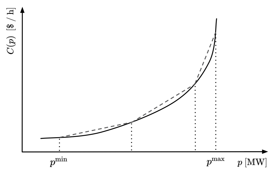 Figure 1. Nonlinear generation cost curve (solid line) and its piecewise linear approximation (dashed lines) by three straight-line segments. \(p^{\mathrm{min}}\) and \(p^{\mathrm{max}}\) specify the operation limits.
Equality constraints
Equality constraints are expressions of the optimization variables characterized by equations.
Equivalently, one can think of an equality constraint as a function of the optimization variables whose function value is fixed.
Because power flow equations express fundamental physical laws, they must naturally be contained in any OPF.
The power balance equations together with the power flow equations \(\eqref{bfm_concise}\) are treated as equality constraints in OPF.
In the equations of power flow, the voltage angle differences play a key role, rather than the individual angles.
Therefore, without loss of generality we can select a specific value of the voltage angle of a bus as reference and apply an additional equality constraint to this reference bus by setting its voltage angle to zero.
We call this the slack or reference bus.
In a more general setting, there can be multiple slack buses (i.e. buses used to make up any generation and demand mismatch caused by line losses) and corresponding constraints on their voltage angle.
Denoting the set of all reference/slack buses by \(\mathcal{R}\) we can write the corresponding constraints for all \(r \in \mathcal{R}\) as: \(\delta_{r} = 0\).
Inequality constraints
Finally, OPF also includes a set of inequality constraints.
Similarly to equality constraints, an inequality constraint can be described by a function of the optimization variables, whose function value is allowed to change within a specified interval.
Inequality constraints usually express some physical limitations of the elements of the system.
For example, the most typical constraints for the ED problem are:
- lower and upper bounds on voltage magnitude of each bus \(i\): \(\underline{v}_{i} \le v_{i} \le \overline{v}_{i}\),
- lower and upper bounds on voltage angle difference between all adjacent buses \(i\) and \(j\): \(\underline{\delta}_{ij} \le \delta_{ij} \le \overline{\delta}_{ij}\),
- lower and upper bounds on output active power of each generator \(g\): \(\underline{p}_{g}^{G} \le p_{g}^{G} \le \overline{p}_{g}^{G}\),
- lower and upper bounds on output reactive power of each generator \(g\): \(\underline{q}_{g}^{G} \le q_{g}^{G} \le \overline{q}_{g}^{G}\),
- upper bounds on the absolute value of active power flow of all transmission lines: \(\lvert p_{ij}\rvert \le \overline{p}_{ij}\),
- upper bounds on the absolute value of reactive power flow of all transmission lines: \(\lvert q_{ij}\rvert \le \overline{q}_{ij}\),
- upper bound on the absolute (square) value of complex power flow of all transmission lines: \(\lvert S_{ij}\rvert^{2} = p_{ij}^{2} + q_{ij}^{2} \le \overline{S}_{ij}^{2}\).
We note that in the actual implementation, some inequality constraints can appear in alternative forms.
For instance, lower and upper bounds on power flows can be replaced by a corresponding set of constraints on the currents.
Solving the ED problem using the interior-point method
Economic dispatch is a non-linear and non-convex optimization problem.
One of the most successful techniques to solve such large-scale optimization problems is the interior-point method.
In this section, we briefly discuss the key aspects of this method.
In a general mathematical optimization, we try to find values of variables \(x\) that minimize an objective function \(f(x)\) subject to a set of equality and inequality constraints \(c^{\mathrm{E}}(x)\) and \(c^{\mathrm{I}}(x)\):
\[\begin{equation}
\begin{aligned}
& \min \limits_{x} \ f(x), \\
& \mathrm{s.t.} \; \; c^{\mathrm{E}}(x) = 0, \\
& \quad \; \; \; \; c^{\mathrm{I}}(x) \ge 0. \\
\end{aligned}
\label{opt_problem}
\end{equation}\]
The ED problem can be expressed in such a form. For example, using the BFM formalism, \(x = X^{\mathrm{BFM}}\), \(\ f(x) = C(X^{\mathrm{BFM}})\), with \(\ c^{\mathrm{E}}_{i} \in \mathcal{C}^{E}\), where \(\mathcal{C}^{\mathrm{E}} = \mathcal{C}^{\mathrm{PB}} \cup \mathcal{C}^{\mathrm{REF}} \cup \mathcal{C}^{\mathrm{BFM}}\), and \(c^{\mathrm{I}}_{j} \in \mathcal{C}^{I}\), where \(\mathcal{C}^{\mathrm{I}} = \mathcal{C}^{\mathrm{INEQ}}\).
Details can be found in the Appendix.
Interior-point methods are also referred to as barrier methods as they introduce a surrogate model of the above optimization problem by converting the inequality constraints to equality ones and replacing the objective function with a logarithmic barrier function:
\[\begin{equation}
\begin{aligned}
& \min \limits_{x, s} \ f(x) - \mu \sum \limits_{i=1}^{\lvert \mathcal{C}^{\mathrm{I}} \rvert} \log s_{i}, \\
& \mathrm{s.t.} \; \; c^{\mathrm{E}}(x) = 0, \\
& \quad \; \; \; \; c^{\mathrm{I}}(x) - s = 0. \\
\end{aligned}
\label{barrier_problem}
\end{equation}\]
Here \(s\) is the vector of slack variables, and the second term in the objective function is called the barrier term, with \(\mu > 0\) barrier parameter.
We note that the barrier term implicitly imposes an inequality constraint on the slack variables, due to the logarithmic function: \(s_i \ge 0\) for all \(i\).
It is easy to see that the barrier problem is not equivalent to the original non-linear program for \(\mu > 0\).
However, as \(\mu \to 0\), the solution of the barrier problem \(\eqref{barrier_problem}\) approaches that of the original optimization problem \(\eqref{opt_problem}\).
The idea of the barrier method is to find an approximate solution of the original problem by using an appropriate sequence of positive barrier parameters that converges to zero.
The basic interior-point algorithm is based on the Karush–Kuhn–Tucker (KKT) conditions of the barrier problem.
The KKT conditions consist of four sets of equations: the first two sets of equations are derived from the first-order condition of the system Lagrangian, i.e. its derivatives with respect to \(x\) and \(s\) are equal to zero, while the third and fourth sets of equations correspond to the equality and inequality constraints, respectively:
\[\begin{equation}
\begin{aligned}
\nabla f(x) - J_{\mathrm{E}}^{T}(x)y - J_{\mathrm{I}}^{T}(x)z = 0, \\
Sz - \mu e = 0, \\
c^{\mathrm{E}}(x) = 0, \\
c^{\mathrm{I}}(x) - s = 0. \\
\end{aligned}
\label{kkt}
\end{equation}\]
The \(J_{\mathrm{E}}(x)\) and \(J_{\mathrm{I}}(x)\) are the Jacobian matrices of the equality and of the inequality functions, and
\(y\) and \(z\) are their corresponding Lagrange multipliers.
Also, we use the following additional notations: \(S = \mathrm{diag}(s)\) and \(Z = \mathrm{diag}(z)\) are diagonal matrices, \(I\) is the identity matrix, and \(e = (1, \dots, 1)^{T}\).
The KKT conditions establish a relationship between the primal \((x, s)\) and dual \((y, z)\) variables, resulting in a non-linear system \(\eqref{kkt}\) that can be expressed by a vector-valued function: \(F_{\mathrm{KKT}}(x, s, y, z) = 0\).
In order to solve this non-linear system, we can apply the Newton–Raphson method and look for a search direction based on the following linear problem:
\[\begin{equation}
J_{\mathrm{KKT}}(x, s, y, z)p \ =\ -F_{\mathrm{KKT}}(x, s, y, z),
\label{primal_dual}
\end{equation}\]
where \(J_{\mathrm{KKT}}(x, s, y, z)\) is the Jacobian matrix of the KKT system, and \(p\) is the search direction vector.
The full form of these components is as follows:
\[\begin{equation}
\begin{aligned}
F_{\mathrm{KKT}}(x, s, y, z) & =
\begin{pmatrix}
\nabla f(x) - J_{\mathrm{E}}^{T}(x)y - J_{\mathrm{I}}^{T}(x)z \\
Sz - \mu e \\
c^{\mathrm{E}}(x) \\
c^{\mathrm{I}}(x) - s \\
\end{pmatrix}, \\
J_{\mathrm{KKT}}(x, s, y, z) & =
\begin{pmatrix}
\nabla_{xx}L & 0 & -J_{\mathrm{E}}^{T}(x) & -J_{\mathrm{I}}^{T}(x) \\
0 & Z & 0 & S \\
J_{\mathrm{E}}(x) & 0 & 0 & 0 \\
J_{\mathrm{I}}(x) & -I & 0 & 0 \\
\end{pmatrix}, \\
p & =
\begin{pmatrix}
p_{x} \\
p_{s} \\
p_{y} \\
p_{z} \\
\end{pmatrix},
\end{aligned}
\end{equation}\]
where the Lagrangian of the system is defined as
\[\begin{equation}
L(x, s, y, z) = f(x) - y^{T} c^{\mathrm{E}}(x) - z^{T} \left( c^{\mathrm{I}}(x) - s \right),
\label{lagrangian}
\end{equation}\]
and \(\nabla_{xx}L\) is the Hessian of the Lagrangian with respect to the optimization variables.
Equation \(\eqref{primal_dual}\)
is called the primal-dual system, as it includes the dual variables besides the primal ones.
The primal-dual system is solved iteratively: in iteration \((n+1)\), after obtaining \(p^{(n+1)}\), we can update the variables \((x,s,y,z)\) and the barrier parameter \(\mu\):
\[\begin{equation}
\begin{aligned}
& x_{n+1} = x_{n} + \alpha_{x}^{(n+1)} p_{x}^{(n+1)}, \\
& s_{n+1} = s_{n} + \alpha_{s}^{(n+1)} p_{s}^{(n+1)}, \\
& y_{n+1} = y_{n} + \alpha_{y}^{(n+1)} p_{y}^{(n+1)}, \\
& z_{n+1} = z_{n} + \alpha_{z}^{(n+1)} p_{z}^{(n+1),} \\
& \mu_{n+1} = g(\mu_{n}, x_{n+1}, s_{n+1}, y_{n+1}, z_{n+1}), \\
\end{aligned}
\end{equation}\]
where \(g\) is a function that computes the next value of \(\mu\)
from the previous value and the updated variables.
The \(\alpha_k\)’s are line search parameters for variables \(k = x, s, y, z\)
that are dynamically adapted to get better convergence.
There are several modern interior-point methods that propose different heuristic functions for computing line search parameters \(\alpha_k\) and barrier parameter \(\mu\), in order to cope with non-convexities and non-linearities, and to provide good convergence rates.
OPF variants
So far we have been focusing on one specific OPF problem, a variant of the economic dispatch that is one of the most basic types in the realm of OPF.
In this section, we briefly discuss other models.
In a more general setting, the task of economic dispatch is to optimize some economic utility function for participants, including both loads and generators.
For instance, incorporating both power supply and power demand into the objective function leads to the basic concept of the electricity market.
At the optimum, the amount of supply and demand power reflects simple market principles subject to the physical constraints of the system: power is primarily bought from generators offering the lowest prices and primarily sold to loads offering the highest prices.
In the so-called volt/var control we optimize the combination of power loss, peak demand, and power consumption, with respect to the voltage level and reactive powers.
In the above problems, the set of generators is specified and all of these generators are supposed to contribute to the total power generation.
However, in real industrial problems, not all generators in the grid need to be active.
Generators differ in many ways besides their generation curve: they have different start up and shut down time scales (i.e. how quickly a generator can reach its operating level and how quickly it can stop running), different costs and ramp rates (i.e. the rates at which a generator can increase or decrease its output), different minimum and maximum power generation, etc. All of these quantities need to be taken into account in the planning procedure.
Therefore, it is very much desirable to allow specific generators to not run in the optimization model.
In order to select the active generators, electricity grid operators solve the unit commitment (UC) problem.
The unit commitment economic dispatch (UCED) problem can be considered an extension of the ED problem, where the set of variables is extended with binary variables, each responsible for including or excluding a specific generator in the optimization.
The UC problem is, therefore, a mixed-integer non-linear programming problem, which is even harder to solve computationally.
Another aspect that needs to be considered is the security of the grid.
Power grids are complex systems that include thousands of buses and transmission lines, where failure of any element can happen occasionally and impact the operation of the power grid significantly.
Thus, it is very important to account for such contingencies.
The corresponding set of problems is called security constrained optimal power flow (SCOPF) and in combination with ED it is called security constrained economic dispatch (SCED).
SCOPF provides a solution not only for the ideal unfailing case, but at the same time for some contingency scenarios as well.
These problems are much larger scale problems, including a much larger number of variables and constraints, and requiring costly mixed-integer non-linear programming.
For example, the widely used \(N-1\) contingency problem addresses all scenarios where a single component fails.
Finally, we note that a more general (and very large-scale) problem can be formulated by using both UC and SCOPF, leading to the security constrained unit commitment problem (SCUC).
Solving OPF problems
Solving OPF problems by interior-point methods, as described earlier, is widely used as a reliable standard approach.
However, solving such problems by interior-point methods is not cheap, as it requires the computation of the Hessian of the Lagrangian \(\nabla_{xx} L(x_{n}, s_{n}, y_{n}, z_{n})\) at each iteration step \(n\) as in equation \(\eqref{primal_dual}\).
Because the required computational time has a disadvantageous superlinear scaling with system size, solving large scale problems can be prohibitively difficult.
Moreover, the scaling is even worse for mixed-integer OPF problems.
There are several approaches that address this issue by either simplifying the original OPF problem, or by computing approximate solutions.
Convex relaxations
The first set of approximations we discuss is called convex relaxations.
The main idea of these approaches is to approximate the original non-convex optimization problem with a convex one.
Unlike in non-convex problems, in convex problems any local minimum is a global minimum as well (so convex problems, by definition, can only have a single minimum).
There are very straightforward algorithms with excellent convergence rates to solve convex optimization problems.
To demonstrate convex relaxations, let us consider the economic dispatch problem with the basic BIM formulation.
As it can be shown, this problem – with some slight modification – can be reformulated as a quadratically constrained quadratic program (QCQP) using the complex voltages of the buses.
In this reformulated optimization problem, the objective function and all (inequality) constraints have a quadratic form in the complex voltages:
\[\begin{equation}
\begin{aligned}
& \min \limits_{V \in \mathbb{C}^{N}}\ V^{H}CV, \\
& \mathrm{s.t.} \quad V^{H}M_{k}V \le m_{k} \quad k \in \mathcal{K}, \\
\end{aligned}
\label{qcqp}
\end{equation}\]
where the superscript \(H\) denotes conjugate transpose, \(M_{k}\)s are Hermitian matrices (i.e.\ \(M_{k}^{H} = M_{k}\)), and \(m_{k}\)s are real-valued vectors specifying the corresponding inequality constraints.
QCQP is still a non-convex problem that is also an NP-hard problem.
Let \(W = VV^{H}\) denote a rank–1 positive semidefinite matrix (i.e. rank\((W) = 1\) and \(W \succeq 0\)).
Using the identity of the trace function for any Hermitian matrix: \(V^{H}MV = \mathrm{tr}(MVV^{H}) = \mathrm{tr}(MW)\), we can transform the quadratic forms of problem \(\eqref{qcqp}\) to expressions that include \(W\) instead of \(V\):
\[\begin{equation}
\begin{aligned}
& \min \limits_{W \in \mathbb{S}}\ \mathrm{tr}(CW), \\
& \mathrm{s.t.} \; \; \mathrm{tr}(M_{k}W) \le m_{k} \quad k \in \mathcal{K}, \\
& \quad \quad \ W \succeq 0, \\
& \quad \quad \ \mathrm{rank}(W) = 1, \\
\end{aligned}
\end{equation}\]
where \(\mathbb{S}\) denotes the space of \(N \times N\) symmetric matrices.
The above problem is convex in \(W\), except for the rank–1 equality constraint.
Removing this constraint leads to a semidefinite programming problem (SDP), which is called the SDP relaxation of the OPF.
SDP introduces a convex superset of the optimization variables.
Other choices of convex supersets yield different relaxations, like chordal or second-order cone programming (SOCP), that can be solved even more efficiently than SDP problems.
We note that all of these relaxations provide a lower bound to OPF.
For some sufficient conditions these relaxations can be even exact.
Also, an advantage of convex relaxation approaches over other approximations is that if a relaxed problem is infeasible, then the original problem is also infeasible.
DC-OPF
One of the most widely used approximations is the DC-OPF approach.
Its name is pretty misleading, as this method does not assume the use of direct current (as opposed to alternating current), although it removes the reactive power flow equations and the corresponding variables and constraints.
The DC approximation is, in fact, a linearization of the original OPF problem (which is sometimes called AC-OPF).
In order to demonstrate the simplifications introduced by the DC-OPF approach, we recall that for a simple power flow model the active and reactive powers flowing from bus \(i\) to \(j\) can be writtes as:
\[\begin{equation}
\left\{
\begin{aligned}
p_{ij} & = \frac{1}{r_{ij}^{2} + x_{ij}^{2}} \left[ r_{ij} \left( v_{i}^{2} - v_{i} v_{j} \cos(\delta_{ij}) \right) + x_{ij} \left( v_{i} v_{j} \sin(\delta_{ij}) \right) \right], \\
q_{ij} & = \frac{1}{r_{ij}^{2} + x_{ij}^{2}} \left[ x_{ij} \left( v_{i}^{2} - v_{i} v_{j} \cos(\delta_{ij}) \right) + r_{ij} \left( v_{i} v_{j} \sin(\delta_{ij}) \right) \right]. \\
\end{aligned}
\right.
\label{power_flow_z}
\end{equation}\]
DC-OPF makes three major assumptions, each of which lead to a simpler expression for the active and reactive power flows (\(p_{ij}\) and \(q_{ij}\)):
- The resistance \(r_{ij}\) of each branch is negligible, i.e. \(r_{ij} \approx 0\).
Applying this assumption to \(\eqref{power_flow_z}\), we obtain:
\[\begin{equation}
\left\{
\begin{aligned}
p_{ij} & {\ \approx\ } \frac{1}{x_{ij}} \left( v_{i}v_{j}\sin(\delta_{ij}) \right) \\
q_{ij} & {\ \approx\ } \frac{1}{x_{ij}} \left( v_{i}^{2} - v_{i} v_{j} \cos(\delta_{ij}) \right)
\end{aligned}
\right.
\end{equation}\]
- The bus voltage magnitudes are approximated by one per unit everywhere, i.e. \(v_{i} \approx 1\).
Using this assumption, we obtain:
\[\begin{equation}
\left\{
\begin{aligned}
p_{ij} & {\ \approx\ } \frac{\sin(\delta_{ij})}{x_{ij}} \\
q_{ij} & {\ \approx\ } \frac{1 - \cos(\delta_{ij})}{x_{ij}}
\end{aligned}
\right.
\end{equation}\]
- The voltage angle difference of each branch is very small, i.e. \(\cos(\delta_{ij}) \approx 1\) and \(\sin(\delta_{ij}) \approx \delta_{ij}\). Applying this assumption leads to our final form:
\[\begin{equation}
\left\{
\begin{aligned}
p_{ij} & {\ \approx\ } \frac{\delta_{ij}}{x_{ij}}, \\
q_{ij} & {\ \approx\ } 0.
\end{aligned}
\right.
\end{equation}\]
As we can see, DC-OPF reduces the original power flow problem significantly by removing several variables and constraints (the full DC-OPF economic dispatch model is shown in the Appendix).
Also, the remaining set of constraints with a linear objective function results in a linear programming problem that can be solved very efficiently by interior-point methods and by simplex methods.
DC-OPF has proven to be useful for a wide variety of applications.
However, it also has several limitations among which the most severe one is that the solution of DC-OPF may not even be a feasible solution of AC-OPF.
In such situations, some constraints need to be tightened, and the DC-OPF computation needs to be re-run.
Computational intelligence and machine learning
The increasing volatility in grid conditions due to the integration of renewable resources (such as wind and solar) creates a desire for OPF problems to be solved in near real-time to have the most accurate state of the system.
Satisfying this desire requires grid operators to have the computational capacity to solve consecutive instances of OPF problems, and do so with fast convergence.
However, this task is rather challenging for large-scale OPF problems—even when using the DC-OPF approximation.
Therefore, as an alternative to interior-point methods, there has been intense research in the computational intelligence and machine learning communities.
Below we provide a list of some well-known approaches.
Computational intelligence techniques for solving OPF:
Among machine learning algorithms, reinforcement, unsupervised, and supervised (both regression and classification) learning approaches can be used to solve OPF problems.
Most of these techniques reduce the computational effort of real-time prediction by performing offline training.
The advantage of taking such an approach is that, while the offline training may be time-consuming, the evaluation of the trained model is typically very fast.
The trained model can be sufficient for a period of time, but may occasionally require re-training.
These machine learning approaches are used for:
- direct prediction of OPF variables;
- prediction of set-points of OPF variables for subsequent warm-starts of interior-point methods;
- prediction of the active constraints of OPF in order to build and solve significantly smaller reduced OPF problems.
In a subsequent blog post, we will talk about using neural networks for some of the above tasks.
Appendix A: the economic dispatch problem using BFM
Putting everything together, the form of the economic dispatch OPF with BFM is as follows:
\[\begin{equation}
\begin{aligned}
& \textbf{Variables:} \\
& \quad X^{\mathrm{BFM}}
\begin{cases}
V_{i} = (v_{i}, \delta_{i}) \hspace{10.4em} \forall i \in \mathcal{N} \\
S_g^{G} = (p_{g}^{G}, q_{g}^{G}) \hspace{9.1em} \forall g \in \mathcal{G} \\
S_{ij} = (p_{ij}, q_{ij}) \hspace{7.8em} \forall (i, j) \in \mathcal{E} \\
S_{ji} = (p_{ji}, q_{ji}) \hspace{7.8em} \forall (j, i) \in \mathcal{E}^{R} \\
I_{ij}^{s} = (i_{ij}^{s}, \gamma_{ij}^{s}) \hspace{8.0em} \forall (i, j) \in \mathcal{E} \\
\end{cases} \\[1em]
& \textbf{Objective function:} \\
& \quad \min \limits_{X^{\mathrm{BFM}}} \sum \limits_{g \in \mathcal{G}} C_{g}(p_{g}^{G}) \\[1em]
& \textbf{Constraints:} \\
& \quad \mathcal{C}^{\mathrm{PB}} \hspace{0.3cm}
\begin{cases}
\sum \limits_{g \in \mathcal{G}_{i}} S_{g}^{G} - \sum \limits_{l \in \mathcal{L}_{i}} S_{l}^{L} - \sum \limits_{s \in \mathcal{S}_{i}} \left( Y_{s}^{S} \right)^{*} \lvert V_{i} \rvert^{2} \\
\hspace{0.95cm} \ = \sum \limits_{(i, j) \in \mathcal{E}} S_{ij} + \sum \limits_{(k, i) \in \mathcal{E}^{R}} S_{ki} \hspace{3.3em} \forall i \in \mathcal{N} \\
\end{cases} \\
& \quad \mathcal{C}^{\mathrm{REF}} \hspace{0.2cm}
\begin{cases}
\delta_{r} = 0 \hspace{1.9cm} \hspace{9.3em} \forall r \in \mathcal{R} \\
\end{cases} \\
& \quad \mathcal{C}^{\mathrm{BFM}} \hspace{0.1cm}
\begin{cases}
I_{ij}^{s} = Y_{ij} \left( \frac{V_{i}}{T_{ij}} - V_{j} \right) \hspace{5.2em} \forall (i, j) \in \mathcal{E} \\
S_{ij} = V_{i} \left( \frac{I_{ij}^{s}}{T_{ij}^{*}} + Y_{ij}^{C} \frac{V_{i}}{\lvert T_{ij} \rvert^{2}}\right)^{*} \hspace{2.6em} \forall (i, j) \in \mathcal{E} \\
S_{ji} = V_{j} \left( -I_{ij}^{s} + Y_{ji}^{C}V_{j} \right)^{*} \hspace{3.0em} \forall (j, i) \in \mathcal{E}^{R} \\
\end{cases} \\
& \quad \mathcal{C}^{\mathrm{INEQ}}
\begin{cases}
\underline{v}_{i} \le v_{i} \le \overline{v}_{i} \hspace{10.1em} \forall i \in \mathcal{N} \\
\underline{p}_{g}^{G} \le p_{g}^{G} \le \overline{p}_{g}^{G} \hspace{9.0em} \forall g \in \mathcal{G} \\
\underline{q}_{g}^{G} \le q_{g}^{G} \le \overline{q}_{g}^{G} \hspace{9.0em} \forall g \in \mathcal{G} \\
\underline{\delta}_{ij} \le \delta_{ij} \le \overline{\delta}_{ij} \hspace{7.6em} \forall (i, j) \in \mathcal{E} \\
\lvert p_{ij}\rvert \le \overline{p}_{ij} \hspace{9.4em} \forall (i, j) \in \mathcal{E} \cup \mathcal{E}^{R} \\
\lvert q_{ij}\rvert \le \overline{q}_{ij} \hspace{9.4em} \forall (i, j) \in \mathcal{E} \cup \mathcal{E}^{R} \\
\lvert S_{ij}\rvert^{2} = p_{ij}^{2} + q_{ij}^{2} \le \overline{S}_{ij}^{2} \hspace{3.9em} \forall (i, j) \in \mathcal{E} \cup \mathcal{E}^{R} \\
\end{cases} \\
\end{aligned}
\label{opf_bmf}
\end{equation}\]
\(\mathcal{C}^{\mathrm{PB}}\), \(\mathcal{C}^{\mathrm{REF}}\), and \(\mathcal{C}^{\mathrm{BFM}}\) denote the equality sets for the power balance, the voltage angle of reference buses, and the improved BFM. \(\mathcal{C}^{\mathrm{INEQ}}\) is the set of inequality constraints.
Appendix B: the DC-OPF economic dispatch problem
\[\begin{equation}
\begin{aligned}
& \textbf{Variables:} \\
& \quad X^{\mathrm{DC}}
\begin{cases}
\delta_{i} \hspace{14.3em} \forall i \in \mathcal{N} \\
p_{g}^{G} \hspace{13.8em} \forall g \in \mathcal{G} \\
p_{ij} \hspace{12.3em} \forall (i, j) \in \mathcal{E} \\
\end{cases} \\[1em]
& \textbf{Objective function:} \\
& \quad \min \limits_{X^{\mathrm{DC}}} \sum \limits_{g \in \mathcal{G}} C_{g}(p_{g}^{G}) \\[1em]
& \textbf{Constraints:} \\
& \quad \mathcal{C}^{\mathrm{PB}} \hspace{0.3cm}
\begin{cases}
\sum \limits_{g \in \mathcal{G}_{i}} p_{g}^{G} - \sum \limits_{l \in \mathcal{L}_{i}} p_{l}^{L} = \sum \limits_{(i, j) \in \mathcal{E}} p_{ij} \hspace{3.4em} \forall i \in \mathcal{N} \\
\end{cases} \\
& \quad \mathcal{C}^{\mathrm{REF}} \hspace{0.15cm}
\begin{cases}
\delta_{r} = 0 \hspace{1.9cm} \hspace{8.5em} \forall r \in \mathcal{R} \\
\end{cases} \\
& \quad \mathcal{C}^{\mathrm{DC}} \hspace{0.3cm}
\begin{cases}
p_{ij} = \frac{\delta_{ij}}{x_{ij}} \hspace{9.4em} \forall (i, j) \in \mathcal{E} \\
\end{cases} \\
& \quad \mathcal{C}^{\mathrm{INEQ}}
\begin{cases}
\underline{v}_{i} \le v_{i} \le \overline{v}_{i} \hspace{9.2em} \forall i \in \mathcal{N} \\
\underline{p}_{g}^{G} \le p_{g}^{G} \le \overline{p}_{g}^{G} \hspace{8.1em} \forall g \in \mathcal{G} \\
\underline{\delta}_{ij} \le \delta_{ij} \le \overline{\delta}_{ij} \hspace{6.7em} \forall (i, j) \in \mathcal{E} \\
\lvert p_{ij}\rvert \le \overline{p}_{ij} \hspace{8.5em} \forall (i, j) \in \mathcal{E} \\
\end{cases} \\
\end{aligned}
\label{opf_dc}
\end{equation}\]
\(\mathcal{C}^{\mathrm{PB}}\), \(\mathcal{C}^{\mathrm{REF}}\), and \(\mathcal{C}^{\mathrm{DC}}\) denote the equality sets for the power balance, the voltage angle of reference buses, and the DC-OPF power flow. \(\mathcal{C}^{\mathrm{INEQ}}\) is the set of inequality constraints.
19 Mar 2021
Author: Eric Perim, Wessel Bruinsma, and Will Tebbutt
In our previous post, we explained that multi-output Gaussian processes (MOGPs) are not fundamentally different from their single-output counterparts. We also introduced the Mixing Model Hierarchy (MMH), which is a broad class of MOGPs that covers several popular and powerful models from the literature. In this post, we will take a closer look at the central model from the MMH, the Instantaneous Linear Mixing Model (ILMM). We will discuss the linear algebra tricks that make inference in this model much cheaper than for general MOGPs. Then, we will take an alternative and more intuitive approach and use it as motivation for a yet better scaling model, the Orthogonal Instantaneous Linear Mixing Model (OILMM). Like most linear MOGPs, the OILMM represents data in a smaller-dimensional subspace; but contrary to most linear MOGPs, in practice the OILMM scales linearly with the dimensionality of this subspace, retaining exact inference.
Check out our previous post for a brief intro to MOGPs. We also recommend checking out the definition of the MMH from that post, but this post should be self-sufficient for those familiar with MOGPs. Some familiarity with linear algebra is also assumed. We start with the definition of the ILMM.
The Instantaneous Linear Mixing Model
Some data sets can exhibit a low-dimensional structure, where the data set presents an intrinsic dimensionality that is significantly lower than the dimensionality of the data. Imagine a data set consisting of coordinates in a 3D space. If the points in this data set form a single straight line, then the data is intrinsically one-dimensional, because each point can be represented by a single number once the supporting line is known. Mathematically, we say that the data lives in a lower dimensional (linear) subspace.
While this lower-dimensionality property may not be exactly true for most real data sets, many large real data sets frequently exhibit approximately low-dimensional structure, as discussed by Udell & Townsend (2019). In such cases, we can represent the data in a lower-dimensional space without losing a significant part of the information. There is a large field in statistics dedicated to identifying suitable lower-dimensional representations of data (e.g. Weinberger & Saul (2004)) and assessing their quality (e.g. Xia et al. (2017)). These dimensionality reduction techniques play an important role in computer vision (see Basri & Jacobs (2003) for an example), and in other fields (a paper by Markovsky (2008) contains an overview).
The Instantaneous Linear Mixing Model (ILMM) is a simple model that appears in many fields, e.g. machine learning (Bonilla et al. (2007) and Dezfouli et al. (2017)), signal processing (Osborne et al. (2008)), and geostatistics (Goovaerts (1997)). The model represents data in a lower-dimensional linear subspace—not unlike PCA— which implies the model’s covariance matrix is low-rank. As we will discuss in the next sections, this low-rank structure can be exploited for efficient inference. In the ILMM, the observations are described as a linear combination of latent processes (i.e. unobserved stochastic processes), which are modelled as single-output GPs.
If we denote our observations as \(y\), the ILMM models the data according to the following generative model: \(y(t) \cond x, H = Hx(t) + \epsilon\). Here, \(y(t) \cond x, H\) is used to denote the value of \(y(t)\) given a known \(H\) and \(x(t)\), \(H\) is a matrix of weights, which we call the mixing matrix, \(\epsilon\) is Gaussian noise, and \(x(t)\) represents the (time-dependent) latent processes, described as independent GPs—note that we use \(x\) here to denote an unobserved (latent) stochastic process, not an input, which is represented by \(t\). Using an ILMM with \(m\) latent processes to model \(p\) outputs, \(y(t)\) is \(p\)-dimensional, \(x(t)\) is \(m\)-dimensional, and \(H\) is a \(p \times m\) matrix. Since the latent processes are GPs, and Gaussian random variables are closed under linear combinations, \(y(t)\) is also a GP. This means that the usual closed-form formulae for inference in GPs can be used. However, naively computing these formulae is not computationally efficient, because a large covariance matrix has to be inverted, which is a significant bottleneck. In the next section we discuss tricks to speed up this inversion.
Leveraging the matrix inversion lemma
When working with GPs, the computational bottleneck is typically the inversion of the covariance matrix over the training input locations. For the case of the ILMM, observing \(p\) outputs, each at \(n\) input locations, we require the inversion of an \(np \times np\) matrix. This operation quickly becomes computationally intractable. What sets the ILMM apart from the general MOGP case is that the covariance matrices generated via an ILMM have some structure that can be exploited.
There is a useful and widely used result from linear algebra that allows us to exploit this structure, known as the matrix inversion lemma (also known as the Sherman–Morrison–Woodbury formula, or simply as the Woodbury matrix formula). This lemma comes in handy whenever we want to invert a matrix that can be written as the sum of a low-rank matrix and a diagonal one. Whereas typically the inversion of such matrices scales with the size of the matrix, the lemma cleverly allows the inversion operation to scale with the rank of the low-rank matrix instead. Therefore, if the rank of the low-rank matrix is much smaller than the size of the matrix, the lemma can enable significant computational speed-ups. We can show that the covariance of the ILMM can be written as a sum of a low-rank and diagonal matrix, which means that the matrix inversion lemma can be applied.
For an ILMM that has \(n\) observations for each of \(p\) outputs and uses \(m\) latent processes, the covariance matrix has size \(np \times np\), but the low-rank part has rank \(nm \times nm\). Thus, by choosing an \(m\) that is smaller than \(p\) and using the matrix inversion lemma, we can effectively decrease the memory and time costs associated with the matrix inversion.
This is not the first time we leverage the matrix inversion lemma to make computations more efficient, see our post on linear models from a GP point of view for another example. The ubiquity of models that represent data in lower-dimensional linear subspaces makes the use of this lemma widespread. However, this approach requires careful application of linear algebra tricks, and obfuscates the reason why it is even possible to get such a speed-up. In the next section we show an alternative view, which is more intuitive and leads to the same performance improvements.
Instead of focusing on linear algebra tricks, let’s try to understand why we can even reduce the complexity of the inversion. The ILMM, as a general GP, scales poorly with the number of observations; and the larger the number of outputs, the larger the number of observations. However, the ILMM makes the modelling assumption that the observations can be represented in a lower-dimensional space. Intuitively, that means that every observation contains a lot of redundant information, because it can be summarised by a much lower-dimensional representation. If it were possible to somehow extract these lower-dimensional representations and use them as observations instead, then that could lead to very appealing computational gains. The challenge here is that we don’t have access to the lower-dimensional representations, but we can try to estimate them.
Recall that the ILMM is a probabilistic model that connects every observation \(y(t)\) to a set of latent, unobserved variables \(x(t)\), defining the lower-dimensional representation. It is this lower-dimensional \(x(t)\) that we want to estimate. A natural choice is to find the maximum likelihood estimate (MLE) \(T(y(t))\) of \(x(t)\) given the observations \(y(t)\):
\[\begin{equation}
T(y(t)) = \underset{x(t)}{\mathrm{argmax}} \, p(y(t) \cond x(t)).
\end{equation}\]
The solution to the equation above is \(T = (H^\top \Sigma^{-1} H)^{-1} H^\top \Sigma^{-1}\) (see prop. 2 of appendix D from Bruinsma et al. (2020)), where \(H\) is the mixing matrix, and \(\Sigma\) is the noise covariance.
The advantage of working with \(Ty(t)\) instead of with \(y(t)\) is that \(y(t)\) comprises \(p\) outputs, while \(Ty(t)\) presents only \(m\) outputs. Thus, conditioning on \(Ty(t)\) is computationally cheaper because \(m < p\). When conditioning on \(n\) observations, this approach brings the memory cost from \(\mathcal{O}(n^2p^2)\) to \(\mathcal{O}(n^2m^2)\), and the time cost from \(\mathcal{O}(n^3p^3)\) to \(\mathcal{O}(n^3m^3)\). These savings are identical to those we get by using the matrix inversion lemma, as discussed in the previous section.
In general, we cannot arbitrarily transform observations and use the resulting transformed data as observations instead. We must show that our proposed procedure is valid, that conditioning on \(Ty(t)\) is equivalent to conditioning on \(y(t)\). We do this showing that (see Bruinsma et al. (2020)), under the ILMM, \(Ty(t)\) is a sufficient statistic for \(x(t)\) given \(y\)—and this is only possible because of the particular structure of the ILMM.
A sufficient statistic \(T(y)\) is a function of the data which is defined with respect to a probabilistic model, \(p(y \cond \theta)\), and an associated unknown parameter \(\theta\). When a statistic is sufficient, it means that computing it over a set of observations, \(y\), provides us with all the information about \(\theta\) that can be extracted from those observations (under that probabilistic model). Thus, there is no other quantity we can compute over \(y\) that will increase our knowledge of \(\theta\). Formally, that is to say that \(p(\theta \cond y) = p(\theta \cond T(y))\). For the ILMM, as \(Ty(t)\) is a sufficient statistic for \(x(t)\), we have that \(p(x(t) \cond y(t)) = p(x(t) \cond Ty(t))\). This property guarantees that the procedure of conditioning the model on the summary of the observations is mathematically valid.
The choice of \(m < p\) is exactly the choice of imposing a low-rank structure onto the model; and the lower the rank (controlled by \(m\), the number of latent processes), the more parsimonious is \(Ty\), the summary of our observations.
Besides being more intuitive, this approach based on the sufficient statistic makes it easy to see how introducing a simple constraint over the mixing matrix \(H\) will allow us to scale the model even further, and obtain linear scaling on the number of latent processes, \(m\). That’s what we discuss next.
The Orthogonal Instantaneous Linear Mixing Model
Although the ILMM scales much better than a general MOGP, the ILMM still has a cubic (quadratic) scaling on \(m\) for time (memory), which quickly becomes intractable for large systems. We therefore want to identify a subset of the ILMMs that scale even more favourably. We show that a very simple restriction over the mixing matrix \(H\) can lead to linear scaling on \(m\) for both time and memory. We call this model the Orthogonal Instantaneous Linear Mixing Model (OILMM). The plots below show a comparison of the time and memory scaling for the ILMM vs the OILMM as \(m\) grows.
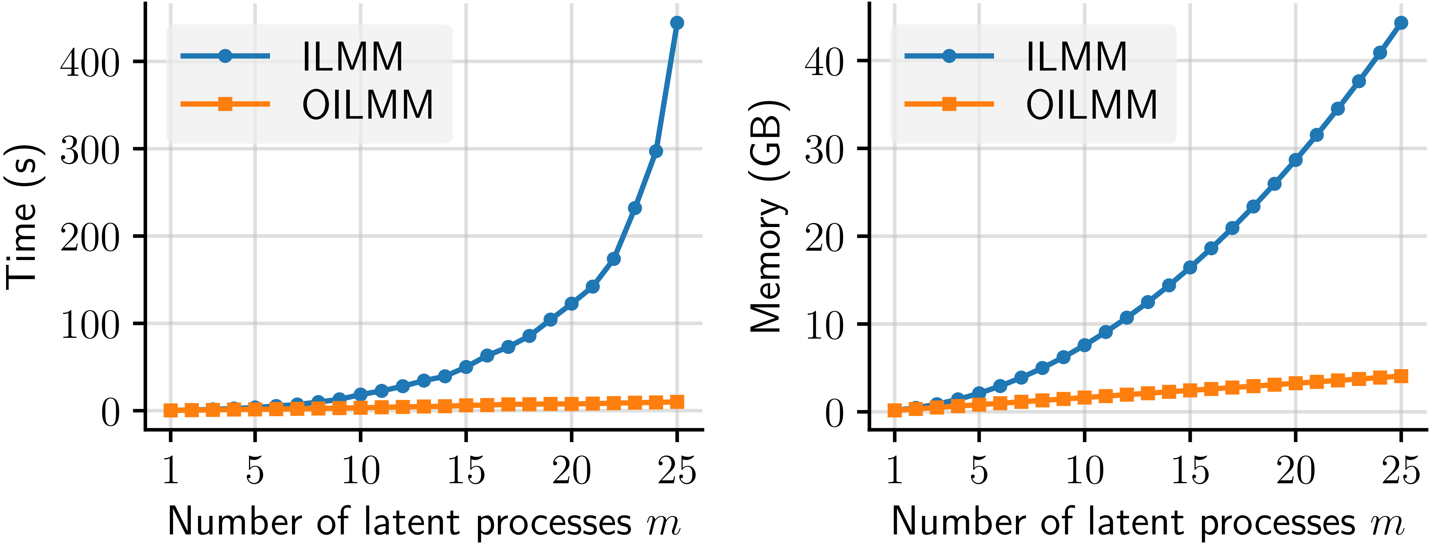 Figure 1: Runtime (left) and memory usage (right) of the ILMM and OILMM for computing the evidence of \(n = 1500\) observations for \(p = 200\) outputs.
Let’s return to the definition of the ILMM, as discussed in the first section: \(y(t) \cond x(t), H = Hx(t) + \epsilon(t)\). Because \(\epsilon(t)\) is Gaussian noise, we can write that \(y(t) \cond x(t), H \sim \mathrm{GP}(Hx(t), \delta_{tt'}\Sigma)\), where \(\delta_{tt'}\) is the Kronecker delta. Because we know that \(Ty(t)\) is a sufficient statistic for \(x(t)\) under this model, we know that \(p(x \cond y(t)) = p(x \cond Ty(t))\). Then what is the distribution of \(Ty(t)\)? A simple calculation gives \(Ty(t) \cond x(t), H \sim \mathrm{GP}(THx(t), \delta_{tt'}T\Sigma T^\top)\). The crucial thing to notice here is that the summarised observations \(Ty(t)\) only couple the latent processes \(x\) via the noise matrix \(T\Sigma T^\top\). If that matrix were diagonal, then observations would not couple the latent processes, and we could condition each of them individually, which is much more computationally efficient.
This is the insight for the Orthogonal Instantaneous Linear Mixing Model (OILMM). If we let \(\Sigma = \sigma^2I_p\), then it can be shown that \(T\Sigma T^\top\) is diagonal if and only if the columns of \(H\) are orthogonal (Prop. 6 from the paper by Bruinsma et al. (2020)), which means that \(H\) can be written as \(H = US^{1/2}\), with \(U\) a matrix of orthonormal columns, and \(S > 0\) diagonal. Because the columns of \(H\) are orthogonal, we name the OILMM orthogonal. In summary: by restricting the columns of the mixing matrix in an ILMM to be orthogonal, we make it possible to treat each latent process as an independent, single-output GP problem.
The result actually is a bit more general: we can allow any observation noise of the form \(\sigma^2I_p + H D H^\top\), with \(D>0\) diagonal. Thus, it is possible to have a non-diagonal noise matrix, i.e., noise that is correlated across different outputs, and still be able to decouple the latent processes and retain all computational gains from the OILMM (which we discuss next).
Computationally, the OILMM approach allows us to go from a cost of \(\mathcal{O}(n^3m^3)\) in time and \(\mathcal{O}(n^2m^2)\) in memory, for a regular ILMM, to \(\mathcal{O}(n^3m)\) in time and \(\mathcal{O}(n^2m)\) in memory. This is because now the problem reduces to \(m\) independent single-output GP problems. The figure below explains the inference process under the ILMM and the OILMM, with the possible paths and the associated costs.
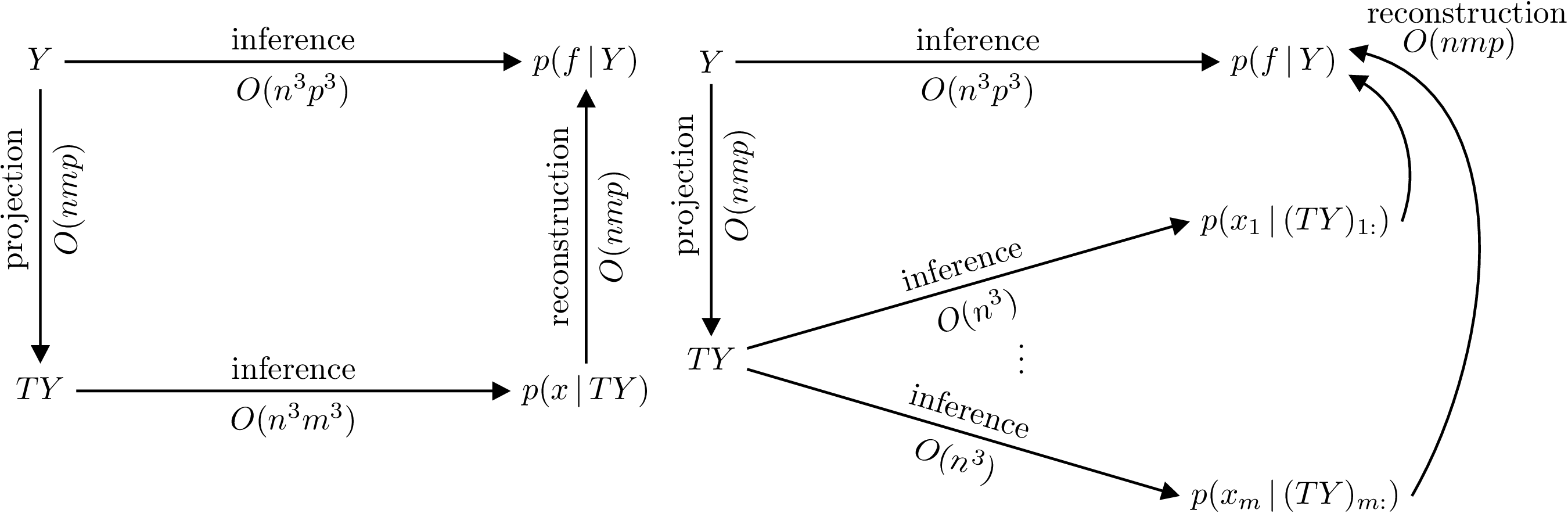 Figure 2: Commutative diagrams depicting that conditioning on \(Y\) in the ILMM (left) and OILMM (right) is equivalent to conditioning respectively on \(TY\) and independently every \(x_i\) on \((TY)_{i:}\), but yield different computational complexities. The reconstruction costs assume computation of the marginals.
If we take the view of an (O)ILMM representing every data point \(y(t)\) via a set of basis vectors \(h_1, \ldots, h_m\) (the columns of the mixing matrix) and a set of time-dependent coefficients \(x_1(t), \ldots, x_m(t)\) (the latent processes), the difference between an ILMM and an OILMM is that in the latter the coordinate system is chosen to be orthogonal, as is common practice in most fields. This insight is illustrated below.
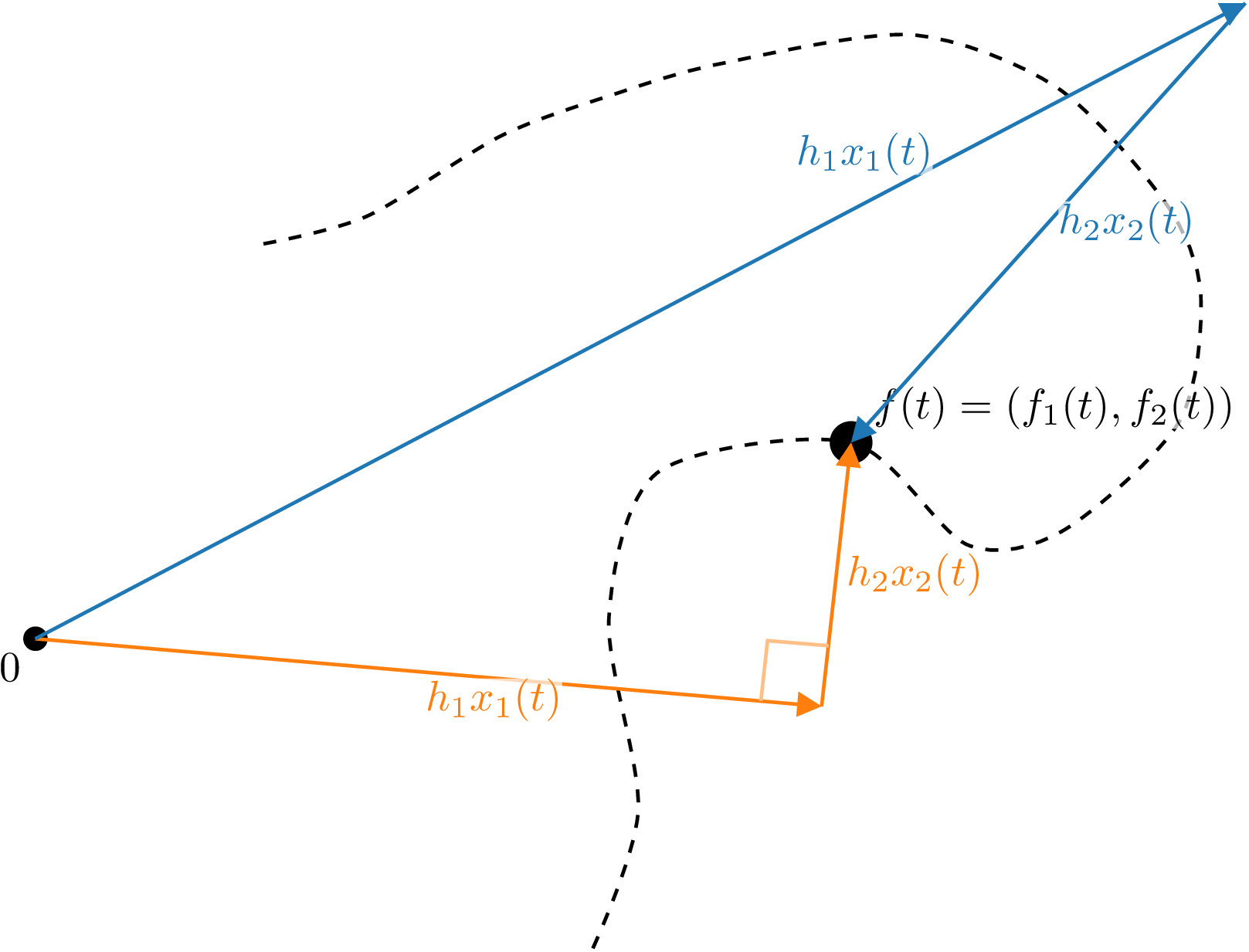 Figure 3: Illustration of the difference between the ILMM and OILMM. The trajectory of a particle (dashed line) in two dimensions is modelled by the ILMM (blue) and OILMM (orange). The noise-free position \(f(t)\) is modelled as a linear combination of basis vectors \(h_1\) and \(h_2\) with coefficients \(x_1(t)\) and \(x_2(t)\) (two independent GPs). In the OILMM, the basis vectors \(h_1\) and \(h_2\) are constrained to be orthogonal; in the ILMM, \(h_1\) and \(h_2\) are unconstrained.
Another important difference between a general ILMM and an OILMM is that, while in both cases the latent processes are independent a priori, only for an OILMM they remain so a posteriori. Besides the computational gains we already mentioned, this property also improves interpretability as the posterior latent marginal distributions can be inspected (and plotted) independently. In comparison, inspecting only the marginal distributions in a general ILMM would neglect the correlations between them, obscuring the interpretation.
Finally, the fact that an OILMM problem is just really a set of single-output GP problems makes the OILMM immediately compatible with any single-output GP approach. This allows us to trivially use powerful approaches, like sparse GPs (as detailed in the paper by Titsias (2009)), or state-space approximations (as presented in the freely available book by Särkkä & Solin), for scaling to extremely large data sets. We have illustrated this by using the OILMM, combined with state-space approximations, to model 70 million data points (see Bruinsma et al. (2020) for details).
Conclusion
In this post we have taken a deeper look into the Instantaneous Linear Mixing Model (ILMM), a widely used multi-output GP (MOGP) model which stands at the base of the Mixing Model Hierarchy (MMH)—which was described in detail in our previous post. We discussed how the matrix inversion lemma can be used to make computations much more efficient. We then showed an alternative but equivalent (and more intuitive) view based on a sufficient statistic for the model. This alternative view gives us a better understanding on why and how these computational gains are possible.
From the sufficient statistic formulation of the ILMM we showed how a simple constraint over one of the model parameters can decouple the MOGP problem into a set of independent single-output GP problems, greatly improving scalability. We call this model the Orthogonal Instantaneous Linear Mixing Model (OILMM), a subset of the ILMM.
In the next and last post in this series, we will discuss implementation details of the OILMM and show some of our implementations in Julia and in Python.
Notes
19 Feb 2021
Author: Eric Perim, Wessel Bruinsma, and Will Tebbutt
This is the first post in a three-part series we are preparing on multi-output Gaussian Processes. Gaussian Processes (GPs) are a popular tool in machine learning, and a technique that we routinely use in our work.
Essentially, GPs are a powerful Bayesian tool for regression problems (which can be extended to classification problems through some modifications).
As a Bayesian approach, GPs provide a natural and automatic mechanism to construct and calibrate uncertainties.
Naturally, getting well-calibrated uncertainties is not easy and depends on a combination of how well the model matches the data and on how much data is available.
Predictions made using GPs are not just point predictions: they are whole probability distributions, which is convenient for downstream tasks. There are several good references for those interested in learning more about the benefits of Bayesian methods, from introductory blog posts to classical books.
In this post (and in the forthcoming ones in this series), we are going to assume that the reader has some level of familiarity with GPs in the single-output setting.
We will try to keep the maths to a minimum, but will rely on mathematical notation whenever that helps making the message clear.
For those who are interested in an introduction to GPs—or just a refresher—we point towards other resources.
For a rigorous and in-depth introduction, the book by Rasmussen and Williams stands as one of the best references (and it is made freely available in electronic form by the authors).
We will start by discussing the extension of GPs from one to multiple dimensions, and review popular (and powerful) approaches from the literature.
In the following posts, we will look further into some powerful tricks that bring improved scalability and will also share some of our code.
Multi-output GPs
While most people with a background in machine learning or statistics are familiar with GPs, it is not uncommon to have only encountered their single-output formulation.
However, many interesting problems require the modelling of multiple outputs instead of just one.
Fortunately, it is simple to extend single-output GPs to multiple outputs, and there are a few different ways of doing so. We will call these constructions multi-output GPs (MOGPs).
An example application of a MOGP might be to predict both temperature and humidity as a function of time. Sometimes we might want to include binary or categorical outputs as well, but in this article we will limit the discussion to real-valued outputs.
(MOGPs are also sometimes called multi-task GPs, in which case an output is instead referred to as a task. But the idea is the same.)
Moreover we will refer to inputs as time, as in the time series setting, but all the discussion in here is valid for any kind of input.
The simplest way to extend GPs to multi-output problems is to model each of the outputs independently, with single-output GPs.
We call this model IGPs (for independent GPs). While conceptually simple, computationally cheap, and easy to implement, this approach fails to account for correlations between outputs.
If the outputs are correlated, knowing one can provide useful information about others (as we illustrate below), so assuming independence can hurt performance and, in many cases, limit it to being used as a baseline.
To define a general MOGP, all we have to do is to also specify how the outputs covary.
Perhaps the simplest way of doing this is by prescribing an additional covariance function (kernel) over outputs, \(k_{\mathrm{o}}(i, j)\), which specifies the covariance between outputs \(i\) and \(j\).
Combining this kernel over outputs with a kernel over inputs, e.g. \(k_{\mathrm{t}}(t, t')\), the full kernel of the MOGP is then given by
\[\begin{equation}
k((i, t), (j, t')) = \operatorname{cov}(f_i(t), f_j(t')) = k_{\mathrm{o}}(i, j) k_{\mathrm{t}}(t, t'),
\end{equation}\]
which says that the covariance between output \(i\) at input \(t\) and output \(j\) at input \(t'\) is equal to the product \(k_{\mathrm{o}}(i, j) k_{\mathrm{t}}(t, t')\).
When the kernel \(k((i, t), (j, t'))\) is a product between a kernel over outputs \(k_{\mathrm{o}}(i, j)\) and a kernel over inputs \(k_{\mathrm{t}}(t,t’)\), the kernel \(k((i, t), (j, t'))\) is called separable.
In the general case, the kernel \(k((i, t), (j, t'))\) does not have to be separable, i.e. it can be any arbitrary positive-definite function.
Contrary to IGPs, general MOGPs do model correlations between outputs, which means that they are able to use observations from one output to better predict another output.
We illustrate this below by contrasting the predictions for two of the outputs in the EEG dataset, one observed and one not observed, using IGPs and another flavour of MOGPs, the ILMM, which we will discuss in detail in the next section. Contrary to the independent GP (IGP), the ILMM is able to successfully predict F2 by exploiting the observations for F3 (and other outputs not shown).
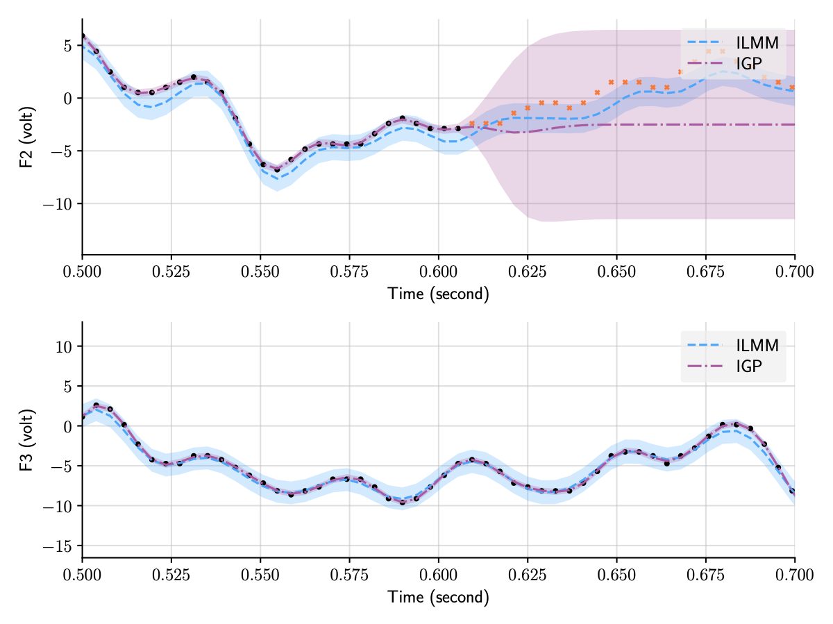 Figure 1: Predictions for two of the outputs in the EEG dataset using two distinct MOGP approaches, the ILMM and the IGP.
All outputs are modelled jointly, but we only plot two of them for clarity.
Figure 1: Predictions for two of the outputs in the EEG dataset using two distinct MOGP approaches, the ILMM and the IGP.
All outputs are modelled jointly, but we only plot two of them for clarity.
Equivalence to single-output GPs
An interesting thing to notice is that a general MOGP kernel is just another kernel, like those used in single-output GPs, but one that now operates on an extended input space (because it also takes in \(i\) and \(j\) as input).
Mathematically, say one wants to model \(p\) outputs over some input space \(\mathcal{T}\).
By also letting the index of the output be part of the input, we can construct this extended input space: \(\mathcal{T}_{\mathrm{ext}} = \{1,...,p\} \times \mathcal{T}\). Then, a multi-output Gaussian process (MOGP) can be defined via a mean function, \(m\colon \mathcal{T}_{\mathrm{ext}} \to \mathbb{R}\), and a kernel, \(k\colon \mathcal{T}_{\mathrm{ext}}^2 \to \mathbb{R}\).
Under this construction it is clear that any property of single-output GPs immediately transfers to MOGPs, because MOGPs can simply be seen as single-output GPs on an extended input space.
An equivalent formulation of MOGPs can be obtained by stacking the multiple outputs into a vector, creating a vector-valued GP.
It is sometimes helpful to view MOGPs from this perspective, in which the multiple outputs are viewed as one multidimensional output.
We can use this equivalent formulation to define MOGP via a vector-valued mean function, \(m\colon \mathcal{T} \to \mathbb{R}^p\), and a matrix-valued kernel, \(k\colon\mathcal{T}^2 \to \mathbb{R}^{p \times p}\). This mean function and kernel are not defined on the extended input space; rather, in this equivalent formulation, they produce multi-valued outputs.
The vector-valued mean function corresponds to the mean of the vector-valued GP, \(m(t) = \mathbb{E}[f(t)]\), and the matrix-valued kernel to the covariance matrix of vector-valued GP, \(k(t, t’) = \mathbb{E}[(f(t) - m(t))(f(t’) - m(t’))^\top]\).
When the matrix-valued kernel is evaluated at \(t = t’\), the resulting matrix \(k(t, t) = \mathbb{E}[(f(t) - m(t))(f(t) - m(t))^\top]\) is sometimes called the instantaneous spatial covariance: it describes a covariance between different outputs at a given point in time \(t\).
Because MOGPs can be viewed as single-output GPs on an extended input space, inference works exactly the same way.
However, by extending the input space we exacerbate the scaling issues inherent with GPs, because the total number of observations is counted by adding the numbers of observations for each output, and GPs scale badly in the number of observations.
While inference in the single-output setting requires the inversion of an \(n \times n\) matrix (where \(n\) is the number of data points), in the case of \(p\) outputs, assuming that at all times all outputs are observed, this turns into the inversion of an \(np \times np\) matrix (assuming the same number of input points for each output as in the single output case), which can quickly become computationally intractable (i.e. not feasible to compute with limited computing power and time).
That is because the inversion of a \(q \times q\) matrix takes \(\mathcal{O}(q^3)\) time and \(\mathcal{O}(q^2)\) memory, meaning that time and memory performance will scale, respectively, cubically and quadratically on the number of points in time, \(n\), and outputs, \(p\).
In practice this scaling characteristic limits the application of this general MOGP formulation to data sets with very few outputs and data points.
Low-rank approximations
A popular and powerful approach to making MOGPs computationally tractable is to impose a low-rank structure over the covariance between outputs.
That is equivalent to assuming that the data can be described by a set of latent (unobserved) Gaussian processes in which the number of these latent processes is fewer than the number of outputs.
This builds a simpler lower-dimensional representation of the data. The structure imposed over the covariance matrices through this lower-dimensional representation of the data can be exploited to perform the inversion operation more efficiently (we are going to discuss in detail one of these cases in the next post of this series).
There are a variety of different ways in which this kind of structure can be imposed, leading to an interesting class of models which we discuss in the next section.
This kind of assumption is typically used to make the method computationally cheaper.
However, these assumptions do bring extra inductive bias to the model. Introducing inductive bias can be a powerful tool in making the model more data-efficient and better-performing in practice, provided that such assumptions are adequate to the particular problem at hand.
For instance, low-rank data occurs naturally in different settings.
This also happens to be true in electricity grids, due to the mathematical structure of the price-forming process.
To make good choices about the kind of inductive bias to use, experience, domain knowledge, and familiarity with the data can be helpful.
The Mixing Model Hierarchy
Models that use a lower-dimensional representation for data have been present in the literature for a long time.
Well-known examples include factor analysis, PCA, and VAEs.
Even if we restrict ourselves to GP-based models there are still a significant number of notable and powerful models that make this simplifying assumption in one way or another.
However, models in the class of MOGPs that explain the data with a lower-dimensional representation are often framed in many distinct ways, which may obscure their relationship and overarching structure.
Thus, it is useful to try to look at all these models under the same light, forming a well-defined family that highlights their similarities and differences.
In one of the appendices of a recent paper of ours, we presented what we called the Mixing Model Hierarchy (MMH), an attempt at a unifying presentation of this large class of MOGP models.
It is important to stress that our goal with the Mixing Model Hierarchy is only to organise a large number of pre-existing models from the literature in a reasonably general way, and not to present new models nor claim ownership over important contributions made by other researchers.
Further down in this article we present a diagram that connects several relevant papers to the models from the MMH.
The simplest model from the Mixing Model Hierarchy is what we call the Instantaneous Linear Mixing Model (ILMM), which, despite its simplicity, is still a rather general way of describing low-rank covariance structures. In this model the observations are described as a linear combination of the latent processes (i.e. unobserved stochastic processes), given by a set of constant weights.
That is, we can write \(f(t) | x, H = Hx(t)\), where \(f\) are the observations, \(H\) is a matrix of weights, which we call the mixing matrix, and \(x(t)\) represents the (time-dependent) latent processes—note that we use \(x\) here to denote an unobserved (latent) stochastic process, not an input, which is represented by \(t\).
If the latent processes \(x(t)\) are described as GPs, then due to the fact that linear combinations of Gaussian variables are also Gaussian, \(f(t)\) will also be a (MO)GP.
The top-left part of the figure below illustrates the graphical model for the ILMM.
The graphical model highlights the two restrictions imposed by the ILMM when compared with a general MOGP: (i) the instantaneous spatial covariance of \(f\), \(\mathbb{E}[f(t) f^\top(t)] = H H^\top\), does not vary with time, because neither \(H\) nor \(K(t, t) = I_m\) varies with time; and (ii) the noise-free observation \(f(t)\) is a function of \(x(t')\) for \(t'=t\) only, meaning that, for example, \(f\) cannot be \(x\) with a delay or a smoothed version of \(x\). Reflecting this, we call the ILMM a time-invariant (due to (i)) and instantaneous (due to (ii)) MOGP.
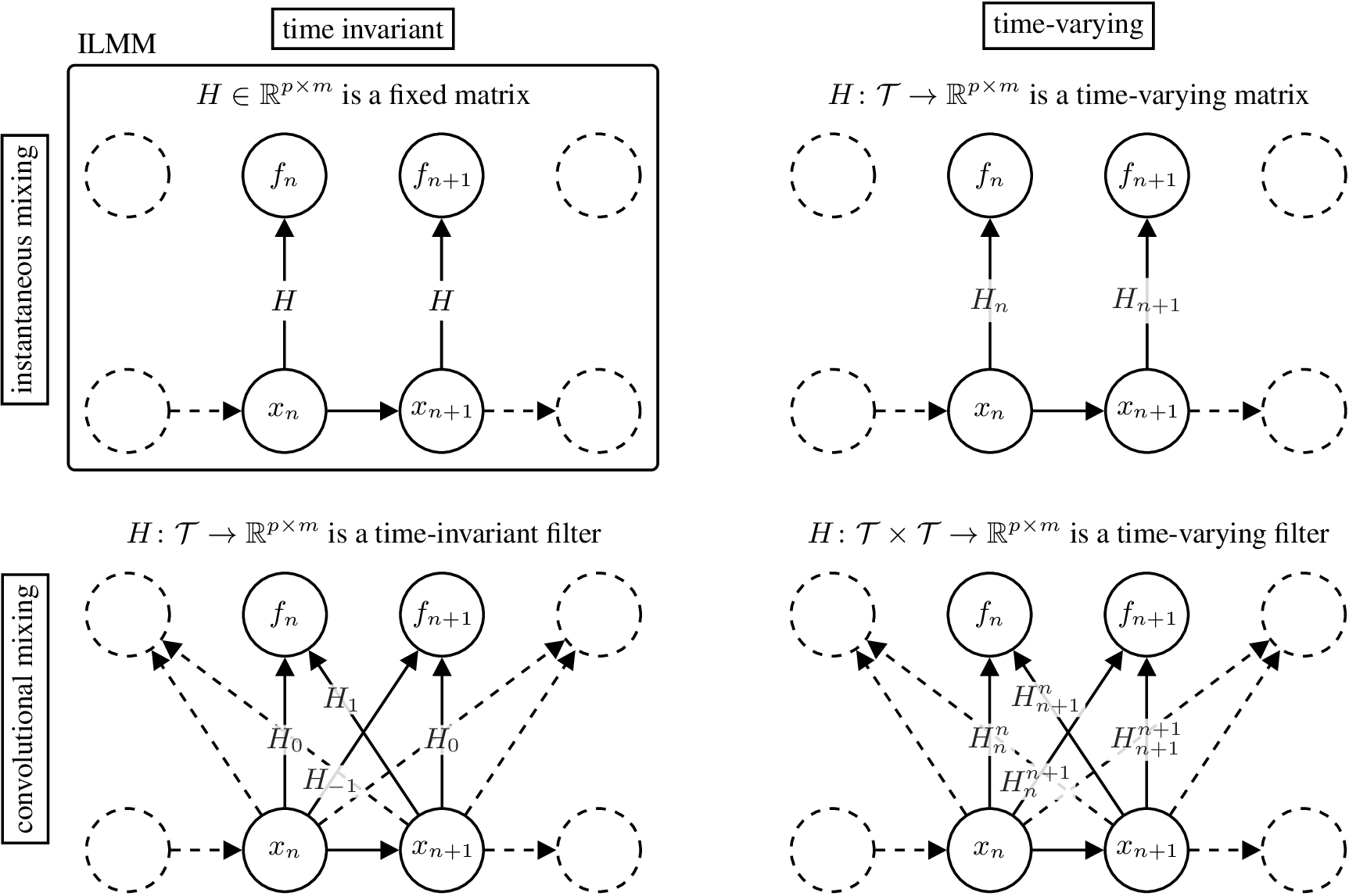 Figure 2: Graphical model for different models in the MMH.
There are three general ways in which we can generalise the ILMM within the MMH.
The first one is to allow the mixing matrix \(H\) to vary in time.
That means that the amount each latent process contributes to each output varies in time.
Mathematically, \(H \in \R^{p \times m}\) becomes a matrix-valued function \(H\colon \mathcal{T} \to \R^{p \times m}\), and the mixing mechanism becomes
\[\begin{equation}
f(t)\cond H, x = H(t) x(t).
\end{equation}\]
We call such MOGP models time-varying.
Their graphical model is shown in the figure above, on the top right corner.
A second way to generalise the ILMM is to assume that \(f(t)\) depends on \(x(t')\) for all \(t' \in \mathcal{T}\).
That is to say that, at a given time, each output may depend on the values of the latent processes at any other time.
We say that these models become non-instantaneous.
The mixing matrix \(H \in \R^{p \times m}\) becomes a matrix-valued time-invariant filter \(H\colon \mathcal{T} \to \R^{p \times m}\), and the mixing mechanism becomes
\[\begin{equation}
f(t)\cond H, x = \int H(t - \tau) x(\tau) \mathrm{d\tau}.
\end{equation}\]
We call such MOGP models convolutional.
Their graphical model is shown in the figure above, in the bottom left corner.
A third generalising assumption that we can make is that \(f(t)\) depends on \(x(t')\) for all \(t' \in \mathcal{T}\) and this relationship may vary with time.
This is similar to the previous case, in that both models are non-instantaneous, but with the difference that this one is also time-varying.
The mixing matrix \(H \in \R^{p \times m}\) becomes a matrix-valued time-varying filter \(H\colon \mathcal{T}\times\mathcal{T} \to \R^{p \times m}\), and the mixing mechanism becomes
\[\begin{equation}
f(t)\cond H, x = \int H(t, \tau) x(\tau) \mathrm{d\tau}.
\end{equation}\]
We call such MOGP models time-varying and convolutional.
Their graphical model is shown in the figure above in the bottom right corner.
Besides these generalising assumptions, a further extension is to adopt a prior over \(H\).
Using such a prior allows for a principled way of further imposing inductive bias by, for instance, encouraging sparsity.
This extension and the three generalisations discussed above together form what we call the Mixing Model Hierarchy (MMH), which is illustrated in the figure below.
The MMH organises multi-output Gaussian process models according to their distinctive modelling assumptions.
The figure below shows how twenty one MOGP models from the machine learning and geostatistics literature can be recovered as special cases of the various generalisations of the ILMM.
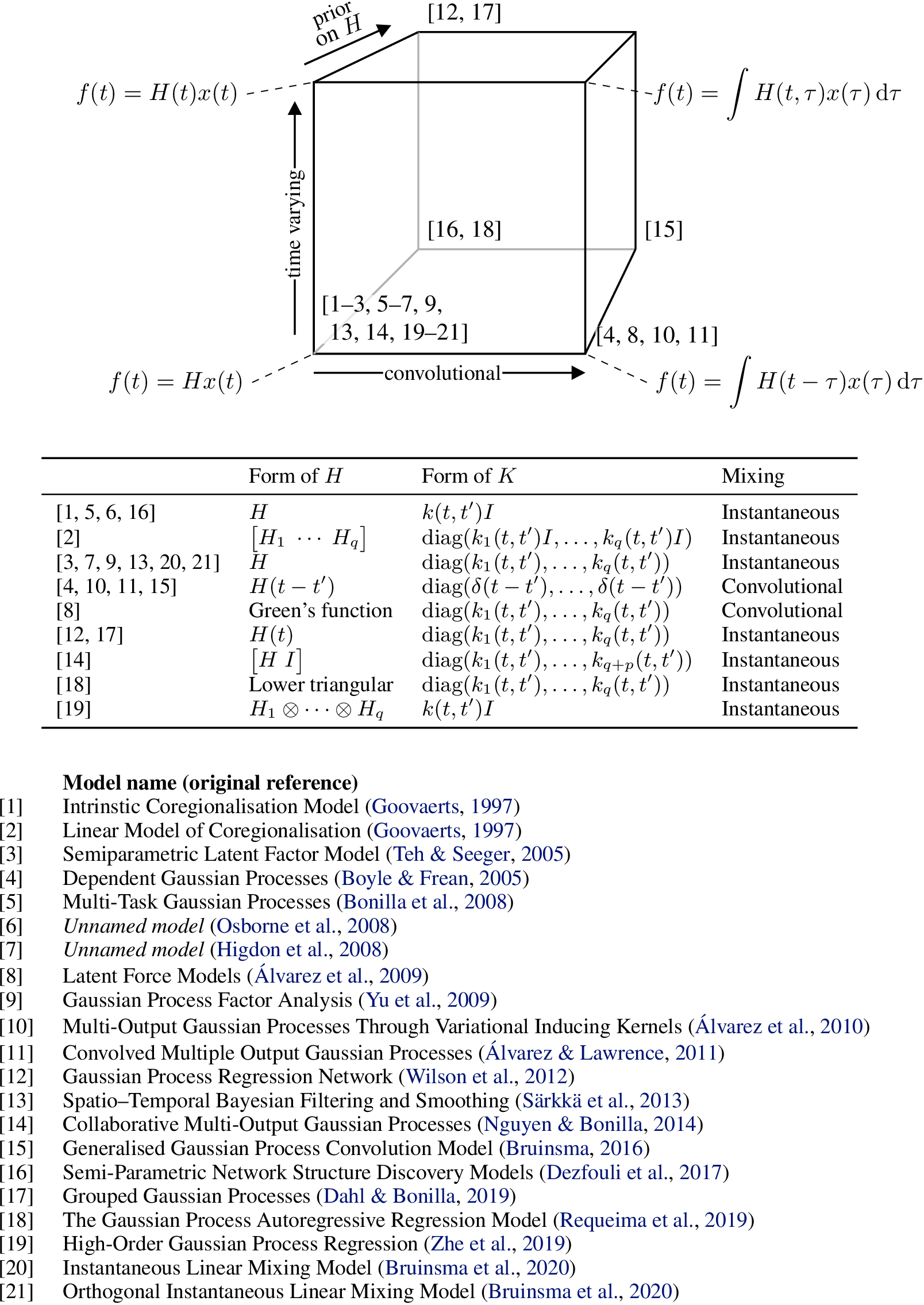 Figure 3: Diagram relating several models from the literature to the MMH, based on their properties.
Naturally, these different members of the MMH vary in complexity and each brings their own set of challenges.
Particularly, exact inference is computationally expensive or even intractable for many models in the MMH, which requires the use of approximate inference methods such as variational inference (VI), or even Markov Chain Monte Carlo (MCMC).
We definitely recommend the reading of the original papers if one is interested in seeing all the clever ways the authors find to perform inference efficiently.
Although the MMH defines a large and powerful family of models, not all multi-output Gaussian process models are covered by it.
For example, Deep GPs and its variations are excluded because they transform the latent processes nonlinearly to generate the observations.
Conclusion
In this post we have briefly discussed how to extend regular, single output Gaussian Processes (GP) to multi-output Gaussian Processes (MOGP), and argued that MOGPs are really just single-output GPs after all.
We have also introduced the Mixing Model Hierarchy (MMH), which classifies a large number of models from the MOGP literature based on the way they generalise a particular base model, the Instantaneous Linear Mixing Model (ILMM).
In the next post of this series, we are going to discuss the ILMM in more detail and show how some simple assumptions can lead to a much more scalable model, which is applicable to extremely large systems that not even the simplest members of the MMH can tackle in general.
Notes
29 Jan 2021
Author: Miha Zgubic
If you are someone who feels comfortable using code to solve a problem, answer a question, or just implement something for fun, chances are you are relying on open source software.
If you want to contribute to open source software, but don’t know how and where to start, this guide is for you.
In this post, we will first discuss some of the possible mental and technical barriers standing between you and your first meaningful contribution.
Then, we will go through the steps involved in making the first contribution.
For the sake of brevity, we assume some basic familiarity with git (if you know how to commit changes and what a branch is, you’ll be fine).
Because many open source projects are hosted on GitHub, we also discuss GitHub Issues, which refer to GitHub functionality that allows discussion about bugs and new features, and the term “pull/merge request” (PR/MR, they are the same thing), which is a mechanism for submitting your changes to be incorporated into the existing repository.
Mental and Technical Barriers
It is easy to observe the world of open source and think:
“Oh look at all these smart people doing meaningful work and developing meaningful relationships, building humanity’s digital heritage that helps to run our civilisation.
I wish I could join the party, but <something I believe to be true>.”
Some misconceptions I and other people have had are listed below, along with what we think about it now.
“I need to be an expert in <the language> AND <the package> to even consider reporting a bug, making a fix, or implementing new functionality.”
If you are using the package and something doesn’t work as expected, you should report it, for example by opening a GitHub issue.
You don’t need to know how the package works internally.
All you need to do is take a quick look at the documentation to see if anything is written about your problem, and check if a similar issue has been opened already.
If you want to fix something yourself, that’s fantastic! Just jump in and try to figure it out.
“I know about <a thing>, but other people know much more, and it’s much better if they implemented it.”
This is almost always the case, unless you are the world’s leading expert on <a thing>.
However, they are likely busy with other important work, and the issue is not a priority for them.
So, either you implement it, or it may not get done at all, so go ahead!
The best part, however, is that these other more knowledgeable people will usually be happy to review your solution and suggest how to make it even better, which means that a great thing gets built and you learn something in the process.
“I don’t know anyone contributing to the package and they look like a team, isn’t it weird if I just jump in and open an issue/PR?”
No, it’s not weird.
Teams make their code and issues public because they’re looking for new contributors like you.
“I won’t be able to create a perfect solution, and people will point out flaws and ask me to change it.”
Solutions to issues usually come in the form of pull requests.
However, opening a PR is best thought of as a conversation about a solution, rather than a finished product that is either approved or rejected.
Experienced contributors often open PRs to solicit feedback about an idea, because an open PR on GitHub offers convenient tools for discussion about code.
Even if you think your solution is complete, people will likely ask you to make changes, and that’s alright!
If it isn’t explicitly mentioned (it should be), ask why the changes are needed—these are valuable opportunities to learn.
“I would like to make a contribution, but don’t know where to start.”
Finding the right place to start can be challenging, but see advice below.
Once you make a contribution or two they will lead you on to others, so you typically only have to overcome this barrier once.
“I know what is broken and I think I know how to fix it, but don’t know the steps to publish these to the official repository.”
That’s fantastic! See the rest of the guide.
“What if people ask for changes? How do I implement those?”
Somehow I thought implementing review feedback was hard and messy, but, in practice, it’s as easy as adding more commits to a branch.
Steps to First Contribution
Now that we have gone through some of the concerns you may have, here is the step-by-step guide to your first contribution.
1) Learn the mechanics of a pull request
The workflow is described in this excellent repository on GitHub, built just for learning the mechanics of making a pull request.
I recommend to go through it by not just reading it, but by actually going through all the steps.
That exercise should make you comfortable with the process.
2) Find something you want to fix
A good first project might be solving a bug that affects you, as that means you already have a test case and you will be more motivated to find a solution.
However, if the bug is in a large and complicated library or requires a lot of code refactoring to fix, it is probably better to start somewhere else.
It may be more enjoyable to start with smaller or medium-sized packages because they can be easier to understand.
When you find a package you would like to modify, make sure that it is the original (not a fork) and it is being maintained, which you can check by looking at the issues and pull requests on its GitHub page.
Then, look through the issues and see if there is something that you find interesting.
Pay attention to good-first-issue labels, which indicate issues that people think are appropriate for first-time contributors.
This usually means that they are nice and not too hard to solve.
You don’t have to restrict yourself to issues good-first-issue labels, feel free to tackle anything you feel motivated and able to do.
Keep in mind that it might be better to start with a smaller PR and get that merged first, before tackling a bigger issue.
You don’t want to submit a week worth of work only to find out that the package has been abandoned and there is nobody willing to review and merge your PR.
When you find an interesting issue and decide you want to work on it, it is a good idea to comment on the issue first and ask whether anyone is willing to review a potential PR.
Commenting will also create a feeling of responsibility and ownership of the issue which will motivate you and help you finish the PR.
As a few ideas, here are some concrete Julia packages that Invenia is involved with, for example AWS.jl for interacting with AWS, Intervals.jl for working with intervals over ordered types, BlockDiagonals.jl for working with block-diagonal matrices, and ChainRules.jl for automatic differentiation.
We are happy to help you contribute to these!
3) Implement your solution, and open a PR
While you should be familiar with the mechanics of pull requests after step 1, there are some additional social/etiquette considerations.
Generally, the authors of open source packages are delighted when someone uses their package, opens issues about bugs or potential improvements, and especially so when someone opens a pull request with a solution to a known problem.
That said, they will appreciate it if you make things easy for them by linking the issue your PR is solving and a brief reason why you have chosen this approach.
If you are unsure about whether something was a good choice, point it out in the description.
If your background isn’t in computer science or software engineering, you might not have heard of unit testing.
Testing is a way of ensuring the correctness of the code by checking the output of the code for a number of inputs.
In packages with unit tests, every new feature is typically expected to come with tests.
When fixing a bug, a test that fails using the old code and passes using the new code may also be expected.
You can make the review process more efficient and pleasant by quickly examining the PR yourself.
What needs to be included in the PR depends on the issue at hand, but there are some general questions you can think about:
- Does my code work in corner cases, did I include reasonable tests?
- Did I add or change documentation to match my changes?
- Does my code formatting follow the rest of the package? Some packages follow code style guides, such as PEP8 or BlueStyle.
- Did I include any lines or files by mistake?
Don’t worry if you can’t answer these questions.
It is perfectly fine to ask!
You can also self-review your PR and add some thoughts as comments to the code.
The contributor’s guide on collaborative practices is a great resource about the best practices regarding collaboration on open source projects.
The packages that follow it display this badge:  Other packages typically have their own guidelines outlined in a file named
 CONTRIBUTING.md.
4) Address feedback, and wait for the merge
Once the PR is submitted someone will likely respond to it in a few days.
If it doesn’t happen, feel free to “bump” it by adding a comment to the PR asking for it to be reviewed.
Most maintainers do not mind if you bump the PR every ten days or so, and in fact find it useful in case it has slipped under their radar.
Ideally the feedback will be constructive, actionable, and educational.
Sometimes it isn’t, and if you are very unlucky the reviewer might come across as stern and critical.
It helps to remember that such feedback might have been unintentional and that you are in fact on the same side, both wanting the best code to be merged.
Using plural first-person pronouns (we) is a good way to convey this sentiment (and remind the reviewer about it), for example:
“What are the benefits if we implement <a feature> in this way?” is better than “Why do you think <a feature> should be implemented this way?”.
Addressing feedback is easy: simply add more commits to the branch that the PR is for.
Once you think you have addressed all the feedback, let the reviewer know explicitly, as they don’t know whether you plan to add more commits or not.
If all went well the reviewer will then merge the PR, hooray!
Conclusions
Unless you have started programming very recently, you likely already have the technical/programming ability to contribute to open source projects.
You have valuable contributions to make, but psychological/sociological barriers may be holding you back.
Hopefully reading this post will help you overcome them: and we are looking forward to welcoming you to the community and seeing what you come up with!
22 Jan 2021
Author: Tom Wright
During the final weeks of my internship with Invenia, while looking back on my time here,
I had the idea to share some thoughts on my experience and what advice I wish I had been given leading up to my start date.
There are countless recipes for a successful internship, and I hope what follows can help guide you towards making yours great.
First and foremost, congratulations on landing your first technical
internship! After hours of fine-tuning your resume, countless cover
letters written, and (if you are in the same boat I was in) having faced
your fair share of rejections, you’ve made it. Before digging into the
rest of this post, take a moment to be proud of the work you’ve put in
and appreciate where it has led you. If perhaps you are reading this in
the middle of your application process and are yet to receive an offer,
don’t worry. The first summer I applied for technical internships, out
of roughly 20 applications sent, I received a single interview and zero
offers. It never feels like it is going to happen until it does. Here’s
a useful
guide
if you’re looking for tips on the application process.
Hopefully the advice that follows in this post will give you some
insight that helps you make a strong impression throughout the course
of your internship. Some more technical subjects or toolkits will be
mentioned for the sake of example, but we won’t get into the details of
these in this post. There are plenty of online resources that provide
great introductions to
git,
the
cloud,
and countless other new topics you might encounter.
Before you start
The most important thing you can do leading up to your internship is try
to relax. It’s common to feel a nervous excitement as your first day
approaches. Remember that you will have plenty of time (give or take 40
hours per week) to focus on this soon enough. Take the time to enjoy
other hobbies or interests while you have the time.
If all distractions fail, a great way to spend any built up excitement
is to do some research. You likely already have a good sense of what the
company does, the general culture and what your role might entail from
the application and interview processes. Feel free to dig deeper into
these topics. See if there’s information on the company website about
your coworkers, the impact your work might drive and the industry as a
whole. This will help you feel more prepared when you start, as well as
settle some jitters in the weeks leading up.
Hitting the ground running
The day has finally arrived, you’ve made it! Surely your first week will
be filled with lots of meetings, introductions, and learning. My advice
for this information overload is about as basic as it gets: take
notes, and lots of them. Ironically, being a software engineer, I am a
big fan of handwriting my notes. I also think it looks better from the
perspective of the person speaking to see someone writing notes by hand
versus typing away at a laptop, unable to see the screen.
In the same vein, any buzzwords you hear (any term, phrase, acronym or
title that you don’t fully understand) should be added to a personal
dictionary. This was really important for me, and I made reference to it
weekly throughout my 8 month internship. You should keep this up
throughout the entire internship, however the first two weeks is likely
when it will grow the most. What is a Docker container and what makes
them helpful? Who knows what [insert some arbitrary industry acronym
here] stands for? These are questions that are super easy to answer by
asking coworkers or even the internet. Maintaining your own shortlist of
important definitions will help fast track your learning and be a great
tool to pass along to new interns that join during your stay.
One of the best ways you can get to know the company and those you are
working with is simply to reach out to your coworkers. This can be
challenging depending on the size of the company you are with. It
becomes even more intimidating if you are in the middle of a global
pandemic and are onboarding from home. Try connecting via Slack, email
or set up calls to get to know those both in and outside of your team.
Learning about the different teams, individuals’ career paths and
building your network is one of the best ways to make the most of your
internship, both personally and professionally. Reaching out like this
can be intimidating, especially early on, but it will show that you are
interested in the company as a whole and highlight that you have strong
initiative. People generally are more than happy to talk about their
work and personal interests. There is no reason not to start this during
your first couple weeks.
The Bulk
Throughout my internship, I discovered three main takeaways that should
be considered by anyone working through an internship, especially if it
is your first.
1. Who is this imposter?
Imposter Syndrome is the feeling of doubting your own skills,
accomplishments and thinking of yourself as some kind of fraud. For me,
this manifested itself as a stream of questions such as When will they
realize they’ve made a huge mistake in hiring me? and thoughts similar
to I am definitely not smart enough for this! Temper this by
remembering they hired you for a reason. After interviewing many
candidates and having spent hours speaking to you and testing your
skills, they picked you. This reminder certainly won’t make all these
anxieties disappear, but can hopefully help mitigate any unnecessary
stress. Being a little nervous can help motivate you to work hard and
push you to succeed. It is worth remembering that all your coworkers
likely went through the same experience, or even still feel this way
from time to time. Feel free to get their insights or experience with
this if you feel comfortable doing so.
These thoughts and feelings might start well before your first day and
last well into the internship itself, as they did in my case. It will
improve with time and experience. Until that happens just
remember to use your available sources of support and try to translate
it into motivation.
2. Asking for help
A big fear I had during my internship was coming across as naive and
inexperienced. I was very worried about asking a question and getting
“How do you not know that? Don’t you know anything?” as a response.
While this is certainly a normal thought process, it is misguided for a
few reasons. First off, my coworkers are great people, as I am sure are
yours. The odds of someone saying that are slim to none, and if they do,
it tells you a lot more about them than it does about you. Secondly, and
this is an important thing to keep in mind: no one expects you to know
everything and be great at everything, especially early on as an
intern. Asking questions is an important part of learning and
internships are no exception. This one comes in two parts: when and how to ask for help.
Let me save you the time I wasted trying to figure out when is the
perfect point to ask a question. While you definitely do not want to
just ask before thinking or doing any digging yourself, no one wants you
endlessly spinning your wheels. Take the time to think about the
problem, see if there are any reliable resources or answers in some
documentation, attempt a couple of solutions, but don’t fuss until the
end of time out of fear of looking dumb.
How you ask for help is the easy one. You’ve done all the work already.
Avoid questions like “Hey how do you do [insert problem]?”, or even
worse “Hey I know this is probably SUPER stupid but I don’t get
[insert problem here] haha!”. Do say something along the lines of
“Hey [insert name]. I have been trying to figure out how to solve
[insert problem] and seem to be stuck. I have tried [insert attempted
solutions] with no success and was hoping you could point me in the
right direction.” You can also frame it as a leading question, such as
“So in order to do X, we have to do Y because of Z?” It doesn’t have
to be a lengthy breakdown of every thought you had, it really shouldn’t
be. People generally prefer concise messages, just show that you have
put some thought and effort into it.
3. Make your voice heard
The scope of this point may vary depending on the size of your company,
its culture and your role, however, the point remains the same. Share
your thoughts on what you are working on. Share what interests you as
subjects, both within and outside your role.
I had the incredible opportunity to contribute to my organization in
ways beyond the scope of my job description. Yes, this is because of the
supportive nature of the company and the flexibility that comes with
working at a smaller organization, but it also would not have happened
had I not shared what I am interested in. I gained fantastic experience
in my role, but also developed an appreciation and better understanding
for other work being done at the company.
Share your thoughts at the weekly team meeting, don’t be afraid to
review code or improve documentation and bounce ideas off coworkers
during coffee breaks (oh, try not to drink too much coffee). They
hired you in large part for your brain, don’t be afraid to use it!
Final Impressions
You’ve made it to the final few weeks of your internship, congrats!
Hopefully you have had a fantastic experience, learning a lot and making
lasting relationships. Now is the time to think of who you would like to
connect with for a chat or call before you finish. This can be for any
number of reasons; giving a little extra thanks, asking for career
advice or even just for the sake of saying farewell to the friends
you’ve made along the way!
Regardless of whether or not you follow any of this advice, I wish you
the best of luck in your internship. While the advice above worked well
for me, it is by no means a one-size-fits-all magical recipe to the
perfect internship. There will certainly be hurdles along the way,
anxieties to overcome, and inevitable mistakes made, all of which will
contribute to making your internship a great learning experience. Good
luck and enjoy the ride.
 Invenia Blog